A Meticulous Guide to Advances in Deep Learning Efficiency over the Years

This post offers a comprehensive and chronological guide to advances in deep learning from the perspective of efficiency: things like clusters, individual hardware, deep learning libraries, compilers — even architectural changes. This post is not a survey paper, and is intended to provide the reader with broader intuition about this field — it would be impossible to include every little detail that has emerged throughout the last 40 years. The posted X thread https://x.com/a1zhang/status/1851963904491950132 also has a very high-level summary of what to expect!

Preface. The field of deep learning has flourished in the past decade to the point where it is hard as both a researcher and a student to keep track of what is going on. Sometimes, I even find it hard to keep track of the actual direction of the field. In a field that often feels hand-wavy and where many methods and results feel lackluster in practice, I wanted to at least get a sense for progress in how we got to where we are now.

I wanted to write this post in a narrative form — to 1) be digestible to the reader rather than an information dump, and 2) allow the reader to view the field from a macroscopic lens and understand why the field moved the way it did. I have tried to be as paper-focused as possible (similar to Lilian Weng style blogs!) and include as many landmark (or just cool) works as I saw fit; if the reader feels something should be included or edited, please let me knowI really hope all of the information is correct and I’ve tried to make sure of it as much as possible, but it is possible I’ve made errors! If you find any, feel free to shoot me an email and let me know! I’m quite a young person, so I was probably playing Minecraft hypixel when some of these breakthroughs happened. Finally, I always recommend reading the original paper when you want to understand something in more depth. There’s no way for me to fit all of the information about every work here (especially the math), so if you’re ever confused and care enough to know the details, I’ve included both citations and a direct link to every mentioned work.! Before we begin, let me just list out some relevant numbers to give us a bit of appreciation for all of the advances to come. I’ve also added some notes for folks who aren’t familiar with what these numbers really mean.

• NVIDIA’s newest Blackwell B200 GPU is estimated to cost 30k – 40k USD.
  • For FP8Recent NVIDIA hardware includes specialized “tensor cores” that can compute matrix multiplication on 8-bit floating point numbers really fast., it can achieve up to ~4500 TeraFLOPSFLOPS means floating-point operations per second, which is a metric for roughly how fast a processor or algorithm is because most operations in deep learning are over floating point numbers., which is absolutely insane!
  • It features 192GB of high-bandwidth memory / DRAM, which is the main GPU memory.
• Llama 3.1 405B, Meta’s latest open-source language model is 405B parameters (~800GB).
  • It was trained on a whopping 16k NVIDIA H100s (sitting on their 24k GPU cluster)
  • It’s training dataset was 15 trillion tokens.

Part I. The Beginning (1980s-2011)

The true beginning of deep learning is hotly contested, but I, somewhat arbitrarily, thought it was best to begin with the first usage of backpropagation for deep learning: Yann Lecun’s CNN on a handwritten digits dataset in 1989.

Backpropagation Applied to Handwritten Zip Code Recognition (Lecun, 1989).
It is remarkable how simple this setup is: given a training dataset of 7291 normalized 16×16 images of handwritten digits, they train a 2-layer convolutional network with 12 5×5 learnable kernels, followed by a final projection to 10 logits. They train for 23 epochs (~3 days), and approximate the Hessian in Newton’s method to perform weight updates. Without an autodifferentiation engine, they had to write their own backpropagation simulator to compute the relevant derivatives. Finally, these experiments were run on a SUN-4/260 work station, which is a single-core machine running at 16.67 MHz and 128MB of RAM.For reference, a Macbook nowadays will have ~2-3 GHz and 16GB of RAM!

Andrej Karpathy has a wonderful blog that attempts to reproduce this paper on modern deep learning libraries with some extra numbers for reference:

• The original model contains roughly 9760 learnable parameters, 64K MACsMAC stands for multiplication-accumulate, which is a common metric for GPUs because they have fused multiply-and-adder instructions for common linear algebra operations, and 1K activations in one forward pass.
• On his Macbook M1 CPU, he trains a roughly equivalent setup in 90 seconds — it goes to show how far the field has progressed!

Some other notable works at the time were the Long Short-Term Memory (1997), Deep Belief Networks (2006), and Restricted Boltsmann Machines (2007), but I couldn’t really find the hardware, software library, or even programming language used to develop these methods (most likely Lisp / CUDA C++). Furthermore, these methods were more concerned with training stability (e.g. vanishing gradient problem) and proving that these methods could converge on non-trivial tasks, so I can only assume “scale” was not really a concern here.

I.1. Existing Fast Linear Algebra Methods

The introduction of the graphics processors in the late 20th century did not immediately accelerate progress in the deep learning community. While we know GPUs and other parallel processors as the primary workhorse of modern deep learning applications, they were originally designed for efficiently rendering polygons and textures in 3D games — for example, if you look at the design of the NVIDIA GeForce 256 (1999), you’ll notice a distinct lack of modern components like shared memoryNot to be confused with shared memory in the OS setting, I think this naming convention is bad. Shared memory on an NVIDIA GPU is a low-latency cache / SRAM that can be accessed among threads in a threadblock. It is typically used to quickly communicate between threads. and tensor cores that are critical for modern deep learning workloads.

Programming a GPU in the 2000s. By this point the CUDA ecosystem had not matured, so the common method for hacking GPUs for general purpose applications was to configure DirectX or OpenGL, the popular graphics APIs at the time, to perform some rendering operation that involved say a matrix multiplication.To corroborate the anecdote above, I had heard that this was true in a talk at Princeton given by Turing award winner Patrick Hanrahan.

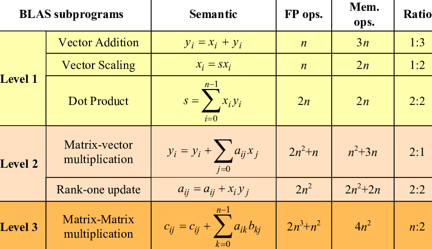
Linear Algebra on a CPU. During this time, a suite of libraries had emerged in parallel for computing and solving common linear algebra paradigms like matrix multiplication, vector addition, dot products, etc. Many of these libraries used or were built off of the BLAS (Basic Linear Algebra Subprograms) specification with bindings for C and Fortran. BLAS divides its routines into three levels, mainly based on their runtime complexity (e.g. level 2 contains matrix-vector operations, which are quadratic with respect to the dimension). On CPUs, these libraries take advantage of SIMD / vectorizationModern CPUs allow for processing multiple elements with a single instruction, enabling a form of parallelization. Hardware components like vector registers (see https://cvw.cac.cornell.edu/vector/hardware/registers) also enable this behavior., smart caching, and multi-threading to maximize throughput. It is also pretty well known that MATLAB, NumPy, and SciPy were popular language / libraries used for these tasks, which essentially used BLAS primitives under the hood. Below were some commonly used libraries:

1. LAPACK (1992): The Linear Algebra Package provides implementations of common linear algebra solvers like eigendecomposition and linear least squares.
2. Intel MKL (1994): The Intel Math Kernel Library is a closed-source library for performing BLAS (now other) operations on x86 CPUs.
3. OpenBLAS (2011): An open-source version of Intel MKL with similar, but worse, performance on most Intel instruction-set architectures (ISAs).
4. OpenCL (2009): An alternative to hacking in OpenGL, OpenCL was a device-agnostic library for performing computations in multiple processors. It was far more flexible for implementing primitives like matrix multiplication.

Just for some reference numbers, I just ran a simple matrix multiplication experiment on my Macbook M2 Pro (12-core CPU, 3.5 GHz) with NumPy 1.26.4, which currently uses OpenBLAS under the hood. I found this blogpost by Aman Salykov which does more extensive experimenting as well.

import numpy as np
import time

SZ = 2048
OPS = SZ * SZ * (2 * SZ – 1)
matrix_a = np.random.rand(SZ, SZ).astype(np.float32)
matrix_b = np.random.rand(SZ, SZ).astype(np.float32)

start_time = time.time()
result = np.dot(matrix_a, matrix_b)
end_time = time.time()

time_taken = end_time – start_time
print(f”Average of {(OPS / time_taken * (1e-9)):.4f} GLOPS”)

> Average of 361.4851 GFLOPS

I.2. Compute Unified Device Architecture (CUDA), 2006

I really like this post by Fabien Sanglard, which explains the history and motivating design patterns of CUDA and NVIDIA GPUs starting from the Tesla architecture over the years.

CUDA was originally designed to enable parallel programmers to work with GPUs without having to deal with graphics APIs. The release of CUDA also came with the release of the NVIDIA Tesla microarchitecture, featuring streaming multiprocessors (SMs), which is the standard abstraction for “GPU cores” used today (this is super important for later!). I’m not an expert in GPU hardware design (actually I’m not an expert in anything for that matter), but the basic idea is that instead of having a lot of complicated hardware units performing specific vectorized tasks, we can divide up computation into general purpose cores (the SMs) that are instead SIMT (single-instruction multiple threads). While this design change was meant for graphics programmers, it eventually made NVIDIA GPUs more flexible for generic scientific workloads.

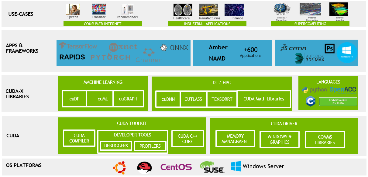
Nowadays, CUDA has evolved beyond just a C API to include several NVIDIA-supported libraries for various workloads. Many recent changes target maximizing tensor core usage, which are specialized cores for fast generalized matrix multiplication (GEMM) in a single cycle. If what I’m saying makes no sense, don’t worry — I will talk more extensively about tensor cores and roughly how CUDA is used with NVIDIA GPUs in the next section.

Some notable libraries that I’ve used in practice are:

• cuBLAS (Introduced in CUDA 8.0): The CUDA API for BLAS primitives.
• cuDNN: The CUDA API for standard deep learning operations (e.g. softmax, activation functions, convolutions, etc.).
• CUTLASS (Introduced in CUDA 9.0): A template abstraction (CuTe layouts) for implementing GEMM for your own kernels — doesn’t have the large overhead of CuBLAS/CuDNN, which supports a wide variety of operations.
• cuSPARSE (Introduced in CUDA 8.0): Efficient linear algebra operations on different kinds of sparse storage formats like coordinate format (COO) and compressed sparse row (CSR).

Part II: Oh s***— Deep learning works! (2012-2020)

Although this section roughly covers the 2010s, many modern methods were derived from works during this time, so you may find some newer techniques mentioned in this section because it felt more natural.

While classical techniques in machine learning and statistics (e.g. SVM, boosting, tree-based methods, kernel-based methods) had been showing promise in a variety of fields such as data science, a lot of people initially did not believe in deep learning. There were definitely people working in the field by the early 2010s, but the pre-dominant experiments were considered more “proof-of-concept”. At the time, classical techniques in fields like computer vision (e.g. SIFT features, edge detectors) and machine translation were thought to be considerably better than any deep-learning methods. That is, until 2012, when team SuperVision dominated every other carefully crafted computer vision technique by an absurd margin.

Part II.1: The first breakthrough on images!

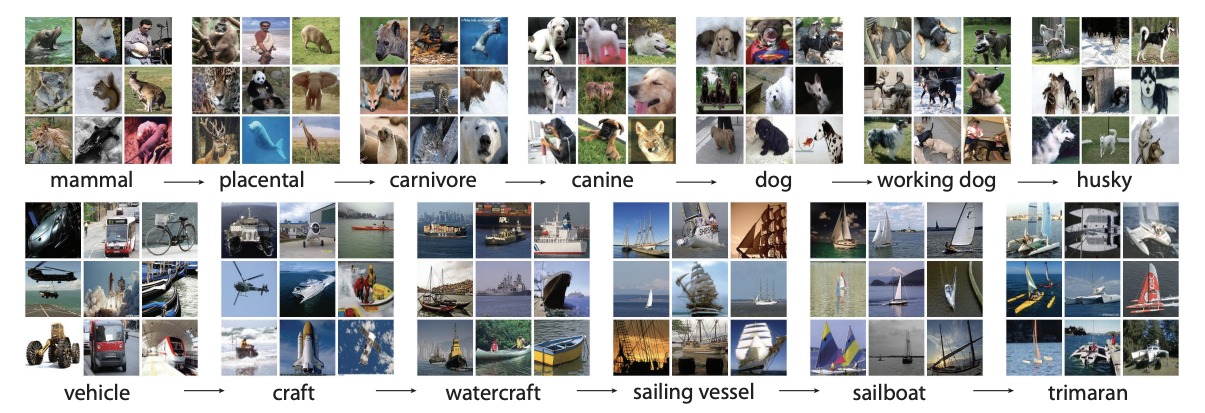
ImageNet, 2009. In 2009, the ImageNet dataset (shout-out to Prof. Kai Li, the co-PI, who is now my advisor at Princeton) was released as “the” canonical visual object recognition benchmark. The dataset itself included over 14 million annotated images with >20k unique classes, and represented the largest annotated image dataset to date. The following is a snippet of 2012 leaderboard for top-5 image classification, where the model is allowed 5 guesses for each image.

ImageNet ILSVRC 2012 Leaderboard for classification, first and second place teams.

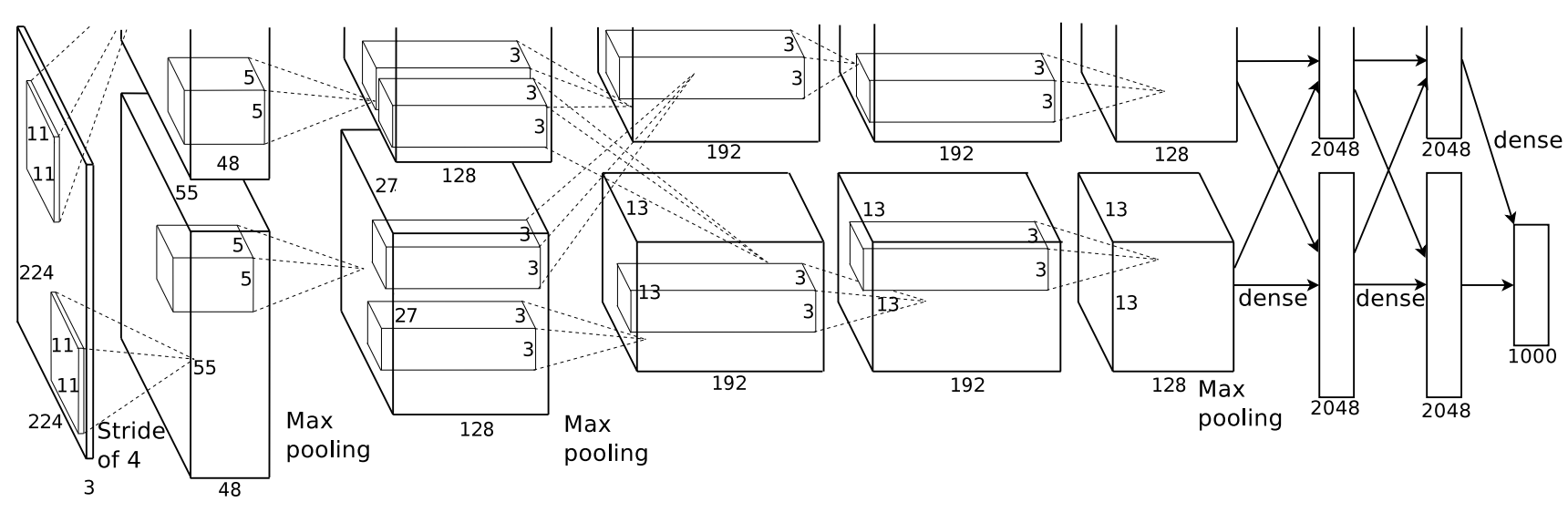
AlexNet (Krizhevsky et al., 2012). AlexNet was one of the first deep convolution networks to be successfully trained on a GPU. The model itself is tiny by today’s standards, but at the time it was far larger than anything that could be trained on a CPU. AlexNet was an 8-layer, 60M parameter model trained on 2 GTX580 GPUs with 3GB of RAM for ~5-6 days. It also featured some important design choices like ReLU activations and dropout that are still common in modern neural networks.

• The original source code in CUDA C++ can be found on Google Code Archive.
• I came across this GitHub repository by user albanie that estimates the throughput of AlexNet’s forward pass to be ~700 MFLOPS, but I’m not sure where they got this runtime estimate from or what hardware it was run on. Regardless, it is most likely an upper-bound for the actual performance.

DanNet (Cireşan, 2011). DanNet was an earlier work by Dan Cireșan in Jürgen Schmidhuber’s lab that similarly implemented a deep convolutional network on GPUs to accelerate training on a variety of tasks. The method itself achieved great performance on a variety of image-based benchmarks, but unfortunately the work is often overshadowed by AlexNet and its success on ImageNet.I want to return to this paper because, while they don’t include the actual hardware used, they mention all the architectural components and dataset details to estimate the efficiency of their approach.

Remark. Interestingly, I found from this Sebastian Raschka blog that there were several other works that had adapted deep neural networks on GPUs. Nonetheless, none of these works had implemented a general-enough method to efficiently scale up the training of a convolutional neural network on the available hardware.

Part II.2: Deep learning frameworks emerge

So it’s 2012, and Alex Krizhevsky, a GPU wizard, has proven that we can successfully use deep learning to blow out the competition on a serious task. As a community, the obvious next step is to build out the infrastructure for deep learning applications so you don’t need to be a GPU wizard to use these tools.

Theano (2012)From what I’m aware of, this library came out earlier, but a lot of the core deep learning features did not come out until 2012.. Theano was an open-source linear algebra compiler developed by the MILA group at Université de Montréal for Python, and it mainly handled optimizing symbolic tensor expressions under the hood. It also handled multi-GPU setups (e.g. data parallelism) without much effort, making it particularly useful for the new wave of deep learning. Personally, I found it quite unintuitive to use by itself, and nowadays it is used as a backend for Keras.

Caffe (2013). Developed at UC Berkeley, Caffe was an older, high-performance library for developing neural networks in C/C++. Models are defined in configuration files, and the focus on performance allowed developers to easily deploy on low-cost machines like edge devices and mobile. Eventually, a lot of features in Caffe/Caffe2 were merged into PyTorch, and by this point it’s rarely directly used.

TensorFlow v1 (2015). Google’s deep learning library targeted Python applications, and felt far more flexible far dealing with the annoying quirks of tensorsTry dealing with tensors in C++ and you’ll quickly see what I mean.. Like its predecessors, TensorFlow v1 also favored a “graph execution” workflow, meaning the developer had to define a computational graph of their models statically so it could be compiled for training / inference. For performance sake, this is obviously a good thing, but it also meant these frameworks were difficult to debug and hard to get used to.

Torch (2002) —> PyTorch (2016). Torch was originally a linear algebra library for Lua, but eventually it evolved into an “eager execution”-basedThe core idea behind eager execution is to execute the model code imperatively. This design paradigm makes the code a lot easier to debug and follow, and is far more “Pythonic” in nature, making it friendly for developers to quickly iterate on their models. deep learning library for Python. PyTorch is maintained as an open-source software, and is arguably the most popular framework used in deep learning research. It used to be the case that you had to touch TorchScript to make PyTorch code production-level fast, but recent additions like torch.compile(), TorchServe, and ONNXONNX was a standard developed jointly by Meta and Microsoft to allow models to be cross-compatible with different frameworks. ONNX is now useful for converting your PyTorch models into other frameworks like Tensorflow for serving. have made PyTorch more widely used in production code as well.

TensorFlow v2 (2019) & Keras (2015). Keras was developed independently by François Chollet, and like PyTorch, it was designed to be intuitive for developers to define and train their models in a modular way. Eventually, Keras merged into TensorFlow, and TensorFlow 2 was released to enable eager execution development in TensorFlow. TensorFlow 2 has a lot of design differences than PyTorch, but I find it relatively easy to use one after you’ve learned the other.

Jax (2020). Google’s latest deep learning framework that emphasizes its functional design and its just-in-time (JIT) XLA compiler for automatically fusing operations (we’ll talk about this more in the GPU section). Jax is more analogous to an amped up NumPy with autodifferentiation features, but it also has support for standard deep learning applications through subsequent libraries like Flax and Haiku. Jax has been getting more popular recently and has, in my opinion, replaced TensorFlow as Google’s primary deep learning framework. Finally, Jax has been optimized heavily for Google’s Tensor Processing Units (TPUs), i.e. anyone using cloud TPUs should be using Jax.

By this point, we’ve set the stage for deep learning to flourish — frameworks are being developed to make research on deep learning far easier, so we can now move on to talking about the types of architectures people were interested in and the core research problems of the time.

Part II.3: New deep learning architectures emerge

Here is where the focus of the field begins to diverge into applying these networks to different domains. For the sake of brevity, I am going to assume the reader is familiar with all of these works, so I will very loosely gloss over what they are. Feel free to skip this section.

Recurrent Networks (1980s – 1990s ish). Recurrent neural networks (RNNs) were popular at the nascent period of deep learning, with methods like GRU and LSTM being used in many time-series and language tasks. Their sequential nature made them hard to scale on parallel processors, making them somewhat obscure for a long time after. More recently, recurrent networks have been re-popularized in the form of state-space models (SSMs) for linear dynamical systems. Early versions of these SSMs used the linear-time-invariance (LTI) assumption to rewrite sequential computations as a convolution at the cost of flexibility. Recent works have removed these assumptions through efficient hardware implementations of critical algorithms like the Fast Fourier Transform.

Convolutional Neural Networks (CNN). CNNs were there from the beginning, and they still remain popular in the computer vision domain. The main component is the convolutional layer, which contains learnable “kernels”Kernel is an annoyingly overloaded term. In this case, it just means a small matrix that is convolved around an input. that are applied through a convolution operation on an N-dimensional input. Convolutional layers are nice because the learned kernels are often somewhat interpretable, and they have built in invariants that work well for learning spatial structure.

Graph Neural Networks. Graph neural networks are somewhat broad, but generally involve some parameterization of a graph using standard deep learning components like a linear weight matrix. They are very hard to implement efficiently on modern hardware (think how locality would be done) and can be very large and sparse. Even though most information can be represented as a graph, in practice there are only certain settings like social media graphs in recommendation systems and biochemistry where they have seen success.

Deep Reinforcement Learning (DRL). DRL generally involved approximating value functions (e.g. DQN) or policies (e.g. PPO) from the RL setting, which were traditionally represented as some kind of discrete key-value map. The standard RL setting is a Markov Decision Process (MDP) with some kind of unknown reward. DRL has also extended to post-training large language models by re-framing the alignment problem as some kind of reward maximization problem. DRL has traditionally also been hard to make efficient because 1) existing algorithms do not respond well to blind scaling, 2) agents interacting with an environment is inherently not parallelizable, 3) the environment itself is a large bottleneck.

Generative Adversarial Networks (Goodfellow et al., 2014). Also hotly contested whether these actually came out in 2014, but GANs were (a rather unstable) framework for training generative models. They had some nice theoretical guarantees (the input distribution is the optimal generator) but ultimately were hard to train, and they also were not great at high-resolution generations.

Diffusion Models (Sohl-Dickstein et al., 2015 & Song et al., 2020). I don’t have intuition as to why diffusion model generations turn out that much better than GANs, but from my own experience they definitely do. A lot of efficiency work in diffusion looks into reducing the number of noise/de-noising steps (which I find counterintuitive to how diffusion even works), and most parameterizations of diffusion models are just standard modules that are used in deep learning (e.g. MLPs, convolutions, transformers, etc.).

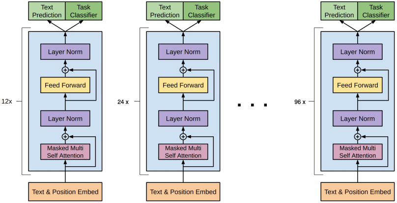
Transformers (Google, 2017). The Transformer block (and variants of it) are widely used today, and a lot of work over the past 5 years has gone into optimizing each component of the Transformer. Some of the key bottlenecks to get around are 1) the quadratic time and memory complexity of the attention mechanism w.r.t sequence length, 2) the growing KV cache that eats up on-device memory, 3) making Transformer computations faster on existing hardware. We will see a lot of these problems come up in the rest of this post.

Part II.4: Efficient convergence. Inductive biases and architectural choices

A natural question any researcher has when first exploring a domain is whether the existing mechanisms and algorithms are optimal. It was known that without tricks like dropout, regularization, the correct activation functions, learning rate scheduler, inductive biases, etc. your model would diverge or overfit on your data. It is way too difficult to pinpoint all of the architectural design changes over the years, and in, for example, the large language space, many of these changes are sort of “open secrets” — many researchers and engineers at large labs are probably aware of these tricks (e.g. local attention, RoPE embeddings, ReLU^2) but as a regular person like myself, it is hard to figure out these details from academic papers. This section will be dedicated to some cool changes that have emerged as empirically useful over the years.

II.4.a: Inductive biases that lead to better convergence behavior

There are many tricks that have been known empirically to lead to better convergence behavior for a lot of models — it is known that many older models struggled to even converge! We still don’t have a rigorous understanding for why many of these tricks are useful, but in this section we list some important architecture changes that have led to better convergence behavior. It’s not always 100% clear why these tricks work so well, so I won’t justify here.

• Dropout (p). During training, randomly mask out $p$. It is believed to be an implicit regularizer.
• Residual connections. First introduced in ResNet, add back the input to the output, effectively allowing data to skip layers.
• Scaling depth/width. For convolutional networks, EfficientNet showed scaling depth/width accordingly is useful.
• Approximating constraints. Optimization over constrained spaces can be annoying. It turns out sometimes relaxing constraints, such as birth of the reinforcement learning algorithm PPO as a relaxed and more widely-used version of TRPO.
• Cosine Learning Rate Scheduler (with Annealing). In NLP settings, the cosine learning rate scheduler (with annealing) is widely used over other fixed and decaying learning rates.
• Loss scaling. To prevent gradients from underflow or overflow (especially for quantization), a lot of optimizers have auto-tuned loss scaling enabled to normalize the gradients, then apply the inverse scaling factor.
• ReLU and variants. For a lot of tasks, especially in NLP, ReLU and its smooth variants seem to work very well as activation functions.
• Adam & AdamW. These momentum-based optimizers have proven to be the most impactful in deep learning despite a lot of research being done in this field.
• Attention. The most famous deep learning mechanism today, attention seems to work very well at interactions over sequential data.
  • RoPE. Rotary embeddings have similar properties to standard positional encodings, but can be written as matrix multiplications (which we love) and work better in a lot of settings.
  • ALiBi. Additive attention biases have proven to work pretty well for length generalization.
• bfloat16. Low-precision training in general has shown to be practical and useful, and the bf16 datatype, which trades of precision for a wider dynamic range than fp16, has shown to be more stable in deep learning training.
• Mixture of Experts. It turns out we can keep scaling our models without all the parameters being active, and we still observe scaling laws.

II.4.b: Searching the space of solutions (meta-optimization)

A lot of traditional machine learning techniques revolve around doing some kind of grid-search and k-folds cross-validation to find the best possible model. In modern deep learning, it’s very hard to do this, especially when a single training run can cost millions of dollars. One of the more interesting spaces is neural architecture search (NAS), where we search a space of model configurations to find models that optimize some metric (e.g. performance, cost, speed) given some set of constraints. NAS isn’t really used in large model training, but it is extremely useful for trying to fit models onto low-cost devices — I’m not sure how much NAS has evolved since 2020, but I would highly recommend reading Lilian Weng’s blog on NAS!

Sakana AI’s Evolutionary Model Merge (Sakana AI, 2024). One of the newer works in NAS for language models is the evolutionary model merge algorithm, which takes components of already trained models and combines them to form various language and multi-modal foundation models. I haven’t played enough with these works to understand how effective they are, but they do demonstrate the ability to create unique models like a Japanese Math LLM with SOTA performance.

Part II.5: Efficient convergence. Optimizers

Recently, I’ve gotten the sense that optimizers are largely overlooked by many people because Adam “just works”. From the perspective of efficiency, if we can 1) compute our optimizers faster, 2) reduce the memory load of stored statistics, and 3) converge faster, then these are all wins to consider. The standard gradient descent update is written as

$$ theta_{t+1} = theta_{t} – eta nabla_{theta} mathcal{L}(theta_t, x^{mathcal{S}}, y^{mathcal{S}}) $$

where $t$ is the iteration, $eta$ is the learning rate, $theta$ is the model parameters, $mathcal{L}$ is the loss function, and $mathcal{S}$ is the set of training values to use in the update. In standard gradient descent (GD), $mathcal{S}$ is the entire dataset, in stochastic gradient descent (SGD) it is a randomly sampled $(x,y)$ pair, and in mini-batch gradient descent it is a randomly sampled subset. While GD has some nice and easy-to-prove theoretical guaranteesIt is quite well known, but look up the proofs for convergence for GD, descent lemma, and even the related empirics surrounding the edge of stability., SGD has similar guarantees and is often used in practice because it converges faster and is easier to compute.

Momentum [intro]. Theoretical guarantees for SGD and GD require knowing the smoothness behavior of the loss function, which in practice is not known. In practice, SGD suffers from “steep” regions in the loss curve that cause oscillatory behavior, motivating the use of the descent trajectory as a prior to dampen oscillations. The canonical momentum update is (where $gamma$ is a constant around $0.9$ according to (Ruder et al. 2016)). The momentum version of SGD introduces a new term that depends on the gradient:

Adam (Kingma and Ba, 2014). It wasn’t mentioned, but Adagrad and RMSprop introduced per-parameter adaptive learning rates and an exponentially decaying average of past gradients. Adam combines these ideas by storing first and second moment estimates of the gradients $g_t$, which is shown in the equations below.The actual Adam also introduces a bias-correcting beta scheduler that modifies the first and second moment estimates slightly. They observed that because the estimates are zero-initialized, they are biased towards 0 if not normalized properly. Furthermore, a variant of Adam, called AdamW, also introduces iterative weight decay and is shown to work well in practice.

From a memory perspective, storing these extra statistics per parameter implies at least an extra 2x the number of model parameters has to be stored in memory during training. For large models, this extra burden is extremely problematic, as we have to figure out 1) how to fit this either into one device’s memory or multiple device’s memory, and 2) if we are using multiple devices, how to move data around effectively. Adam/AdamW is currently the standard for most large language model training as of 2024.

Preconditioning [intro]. Adam has remained the canonical optimizer for a long time, and most people are aware that it is a (stochastic) first-order optimizer. The benefit of a first-order optimizer is that they are relatively quick and only store extra statistics that is linear in the number of learnable parameters. However, it would be a more accurate estimate to use the second, third, etc. order estimates of our loss function Taylor expansion to approximate the correct update. We motivated Adam based on per-coordinate scaling factors, which is basically just applying a diagonal preconditioner to the gradient! Optimizers like Shampoo and Adagrad store preconditioners, but at varying levels of granularity (e.g. block diagonal vs. dense preconditioning matrix). On the AlgoPerf benchmark in particular, Shampoo has been shown to converge quicker than all pre-existing optimizers.

Part II.6: Pause. How much of this scale is really necessary

If you recall how std::vector<T> in the C++ standard library is implemented under the hood, you’ll remember that we have a capacity that marks allocated memory, and a true array size that is the memory that is actually being “used”. This terrible analogy was thought of at 4am just to say that as we continue to scale, a natural question is whether each parameter in the model is really that important.

II.6.a: Model Pruning

Learning both Weights and Connections for Efficient Neural Network (Song et al., 2015). One of the first successful pruning works in deep learning was done for convolutional models (e.g. VGG16, LeNet, AlexNet) on ImageNet. The idea was to first train the models, then zero out weights below a certain norm threshold, then fine-tune the pruned model to completion. They motivate this simple strategy as an implicit regularizer for overfitting, and show ~10x model compression rates while preserving 99% of the performance.

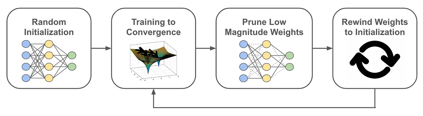
The lottery ticket hypothesis (Frankle et al., 2018). The lottery ticket hypothesis (LTH) is a famous theory that states: for every dense, randomly initialized neural network, there exists a sparse subnetwork that accounts for a majority of the performance. In the original paper, they prune the lowest $N%$ of weights after a certain number of training iterations and show on a variety of image tasks and architectures that performance is preserved. The LTH arguably popularized a lot of derivative works on finding metrics for identifying prunable weights in a network.

SNIP (Lee et al. 2018). The LTH showed that post-training / during-training pruning was more effective than randomly pruning before training, so SNIP proposed a metric to prune “unimportant” weights before training. They first sample a random batch of data $D$ and compute the loss gradients $g_i = frac{partial mathcal{L}(D, theta)}{partial theta_i}$. Then, they compute

$$
S(theta_i) = text{softmax}_{i}left(|g_i(D, theta)|right)
$$

This metric measures how sensitive each weight is to a loss, so they prune the smallest $S(theta_i)$. The authors show that they can prune 99% of a network (LeNet) with a 1% increase in error.

SynFlow (Tanaka et al. 2020). The authors first generalize pruning-at-initialization metrics to what they call “synaptic saliency” as a Hadamard product:

$$
S(theta) = frac{partial mathcal{R}}{partial theta} odot theta
$$

SynFlow was one of the first works to consider pruning from the perspective of “network flow”, as opposed just aggressively pruning weights with a low metric score. They consider scenarios where an entire layer is pruned, leading to a completely redundant network. Their experiments are mainly image models on CIFAR-10/100, but they generally showcase good performance on extreme pruning ratios (on the order of $10^{-3}$).

Are pruned models fast? From a hardware perspective, randomly pruning weights does not provide a large speed-up because operations like weight matrix multiplication rely on locality and targeting blocks of a matrix at one time. The standard implementation is to apply a $0$-mask to each pruned weight – which clearly provides no speed-ups – but clever implementations of pruning can target sparsity-aware kernels like in cuSPARSE and CUTLASSCheck out some of the Han Song lectures like https://www.youtube.com/watch?v=sZzc6tAtTrM&ab_channel=MITHANLab for more information on these topics.. Subsequent works on pruning focus on particular architectures or ensuring hardware-aware speed-ups through structured pruning (e.g. 2:4 pruning). Honestly though, model pruning hasn’t seen that much production-success because 1) many companies can afford to use larger models and 2) pruning generally often is not hardware-friendly, i.e. a 50% pruned model is much slower than a model that is just 50% of the number of parameters.

II.6.b: Embedding Pruning or Hashing

Recommendation systems is a practical field where “pruning” is somewhat applicable. In recommendation systems, users and items are typically represented as an ID that maps to a $O(10)$-dimensional embedding, meaning for social media companies like Meta and Snapchat, they will have on the order of millions or billions of embeddings in their models. For some napkin calculations, a full-precision 1B parameter embedding table with 64-dimensions each is 2 bytes * 64 * 10^9 = 128 GB for the embedding table, which is actually small in production settings! Without going into too much detail about the models themselves (for now, just abstract them as some kind of large transformer model), the embedding tables take up more than 90% of the memory load of learnable parameters.

Intuitively, under a vector space and with some assumptions about constraining the norm of each embedding, it is easy to see that we can probably cluster these embeddings in some meaningful way, and map multiple IDs to the same embedding without incurring much error. Many ideas in RecSys are not shared publicly, but common techniques like double hashing and locality-sensitive hashing are used in practice.

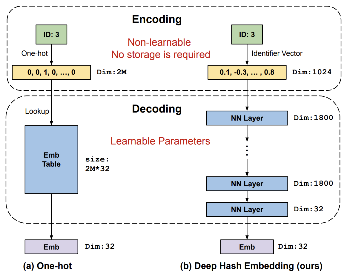
Learning to Embed Categorical Features without Embedding Tables for Recommendation (Kang et al. 2020). Deep Hash Embedding (DHE) is a technique to replace an embedding table with a smaller, learnable transformation (e.g. a neural network). In other words, the hashing function is also implicitly learned alongside the embeddings themselves. Surprisingly, computing embeddings on the fly is pretty effective, but the unclear part for me is whether the values of the IDs have some implicit biasing effect on the embeddings produced.

II.6.c: Quantization

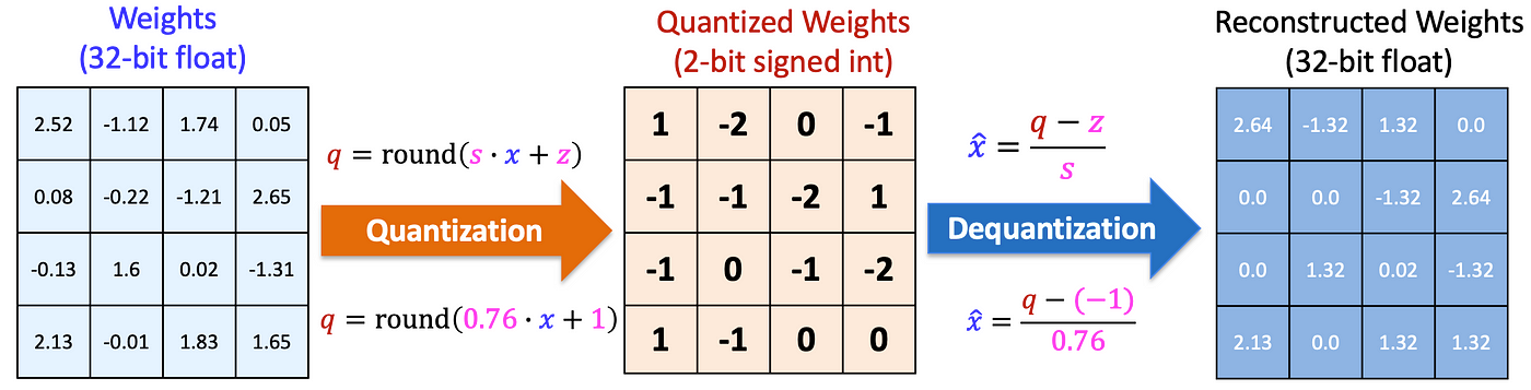
Quantization basically means instead of storing and using 32-bit floating point values (full-precision), we can use maybe 16-bit (half-precision), or 8-bit, etc. Doing so reduces the memory footprint of the model, but at the cost of precision. But there are actually many considerations, like whether you want to quantize during training or after training, whether you want to maintain model computations in a lower precision, and how to handle gradients in mixed-precision models.

The concept of quantization is not specific to deep learning and is more of a data compression problem. Generally, we are interested in reducing the memory footprint of our models — i.e. if we quantize a model with FP32 parameters to INT8FP32 means 32-bit floating point and INT8 means 8-bit integers. We will talk about this a little bit, but they are represented differently in memory. So even INT32 is quite different than FP32., we reduce the model size by 4x. However, as we will see later, modern hardware like the NVIDIA A100 introduces specialized instructions to significantly speed up lower precision operations. For now, we introduce some basic quantization strategies for transforming a value $X$.

Absmax quantization to INT{b} will map to to the closed interval $[- max |X|, max |X|]$ then evenly divide up the interval into $2^b – 1$ sections. Each value will get mapped to its closest point in the above mapping, and the quantization range is clearly symmetric.

$$
X_{int_b} = text{round}left(frac{2^{b-1} – 1}{max |X|} cdot Xright)
$$

Zero-point quantization to INT{b} instead will map to the range $[- min |X|, max |X|]$, but again will still uniformly divide the interval.

The danger of the above methods is the presence of outliers, which cause most quantization bins to be unused while increasing the quantization error. There are many other forms of quantization that do not have to be uniform in any way. Codebook quantization, for example, maps pre-defined values to a smaller set of pre-defined values, and the behavior of this map just has to be injective and well-definedI won’t be going into too much depth about the details of quantizing because it’s not that interesting. I also think that it’s better explained visually. I would recommend reading https://newsletter.maartengrootendorst.com/p/a-visual-guide-to-quantization. The above methods quantize to some integer representation because it is quite intuitive, but quantizing from say FP32 to FP16 is not as obvious because these representations do not uniformly divide the range they represent.

IEEE754 and floating point representations. Integers are represented with the two’s complement and are evenly spaced; however, floating point values are not evenly spaced fractions. Instead, the IEEE754 standard uses one bit to determine sign, some of the bits as exponents, and some of them as fractions (called the mantissa), giving usThere are also special representations for values like $0$ of $infty$, but honestly it’s not that important for us to understand.:

$$
X_{fp32} = s^{(1)} cdot 1.m^{(23)} cdot 2^{b^{(8)}}
$$

I’ve used the superscript to denote the number of bits used to represent that number. To clarify, the mantissa is the decimal part of the number $1.x$. In other words, in FP32, we have $23$ mantissa bits and $8$ exponent bits. However, other representations also exist to modify the representable range (increase exponent bits) or the precision (increase mantissa bits), which can be beneficial in deep learning applications.

• BF16. The IEEE754 standard for FP16 uses 5 exponent bits and 8 mantissa bits. It was discovered by the Google Brain team, however, that using 8 exponent bits, which has the same dynamic range as FP32, was more stable than FP16 due to large gradients in LLM training. Furthermore, BF16 has the benefit of being able to easily convert to and from FP32 — just chop the last 16 bits of the mantissa!
• FP8. NVIDIA’s newest H100s have Tensor Core support for 8-bit floating points, which are represented as either E5M2 or E4M3E5M2 meaning 5 exponent bits and 2 mantissa bits, and E4M3 meaning 4 exponent bits and 2 mantissa bits. Notice that with 8 bits, we can never do the FP32 → BF16 trick, but we can go from FP16 to E5M2.. We will talk more about Tensor Cores soon.

Automatic Mixed-Precision training (2018). In 2018, NVIDIA released the Apex extension to PyTorch, which introduced automatic mixed-precision (AMP) training on CUDA devices. The core idea is that lower precision BLAS operations are significantly faster with the introduction of hardware units like NVIDIA Tensor Cores, but not all operations (e.g. logarithms, trig functions) are safe to downcast due to their sensitivity to dynamic ranges / precision. Under the hood, torch.amp has a list of “safe” operations that are downcast to FP16/BF16 to provide essentially free speed-ups to the programmer. In most modern training schemes, you should be using AMP unless you want full control over your model operations.

II.6.d: The Grandfather of Efficient ML and TinyML

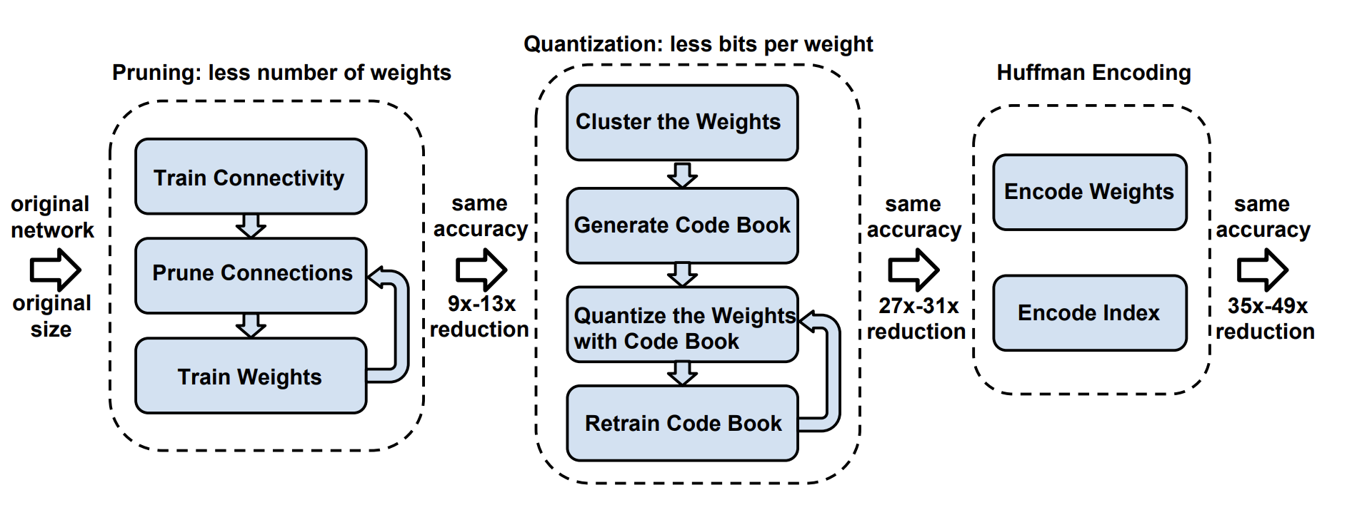
Deep Compression: Compressing Deep Neural Networks with Pruning, Trained Quantization, and Huffman Coding (Han et al. 2015). Arguably the most influential work in efficient deep learning for its time, this paper showed that combining simple magnitude-based weight pruning and codebook quantization was sufficient for cutting down existing images models like VGG-16 by ~50x while barely affecting model performance, enabling them to fit into on-chip SRAM. I wish there was some more analysis on the properties of these extremely compressed models and how this relates to the data distribution the model was trained on, because we do not see these levels of compression in modern LLMs.

Part II.x: Hardware

If you don’t know anything about a GPU except that it’s really good at parallel workloads, this section is a gold mine of information! I think this section motivates a lot of the future work very well, especially as we begin to consider hardware-aware algorithms for scaling our models. Otherwise, I would skip ahead to Chapter III.

You’ve probably noticed that up until this point, a lot of the aforementioned works were interested in improving and tweaking architectural components for the sake of better convergence behavior and ease of scaling. If your model doesn’t fit on a single GPU, find a way to divvy it up on multiple GPUs — we can sort of ignore optimizing for memory accesses, node-to-node latency, and other systems-y lingo because at this scale, it’s probably fast enoughThis isn’t entirely true, of course. There were definitely people who cared about these kinds of “engineering” problems, but AI wasn’t really a “product” yet. It was cool, and it had a growing list of applications, but nothing at the scale of a Google search engine or a streaming platform. . But as the field began to mature, people began thinking more about hardware-aware algorithms and how to utilize a lot of the new features offered by the CUDA ecosystem and NVIDIA GPUs. We focus a lot on CUDA because of its strong support in most deep learning applications, but also recognize and discuss other alternatives.

II.x.1: NVIDIA GPUs from Tesla (2006) to Ampere (2020)

Let’s continue where we left off. A lot of this section will appear kind of hand-wavy, but don’t worry — it makes a lot of sense to just assume things are a certain way before digging into why. If you ever become interested in the why, you’ll have to start reading denser sources of information. I recommend the PPMP textbook and the GPU MODE Discord!

Compute Structure. Let’s first talk about why GPUs are so good at parallelized computations. CPUs were designed to handle very complicated logic like branching (think if-else operations), and a large portion of the processor die is dedicated to this. NVIDIA GPUs instead trade off this chip space for more cores and specific hardware units that can perform instructions like small matrix multiplications in very few cycles. It’s like having 100 automatic sewing robots (GPU) vs. a human (CPU). Sure, the human being is smarter and more flexible/capable for general tasks, but if the task is to maximize production of clothes, it is much more useful to have the sewing robots. Starting from the Tesla series GPUs, NVIDIA used many CUDA cores with the SIMT (single-instruction, multiple threads) abstraction, so effectively a GPU really was just a bunch of small processors running in parallel. To understand how this abstraction works together with actual workloads, however, we need to understand how data is moved from the memory to the actual processors.

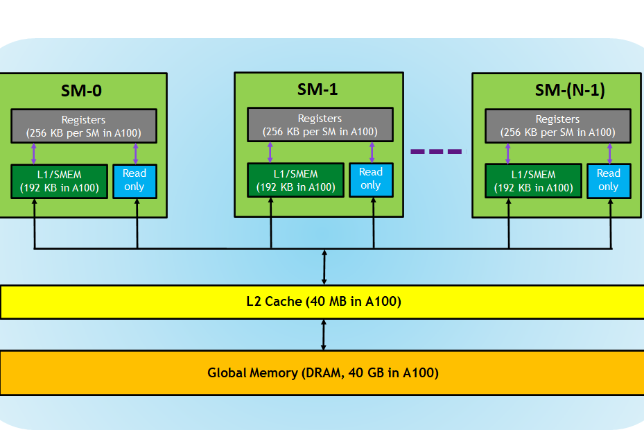
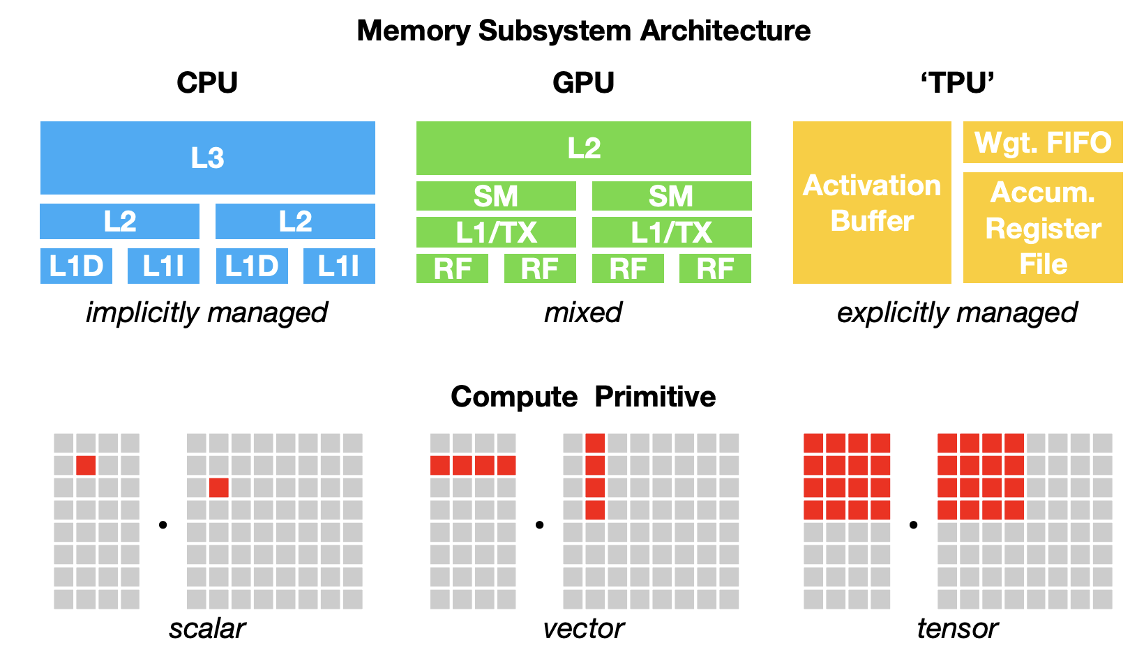
Hierarchical Memory Structure. The above is an extremely simplified view of how compute and memory are divided in a GPU starting from the Tesla architecture. Let’s assume that performing some kind of memory access from global memory (DRAM) is slow. This design emphasizes data reuse to minimize access to global memory. From Figure 12, we can also observe that different hierarchies of memory are shared across different abstractions (e.g. L2 cache is shared among SMs, but L1 cache is per SM), which is extremely important for optimization.

• SMs (streaming multiprocessors) are the individual units that run their own processesThis is not entirely true. SMs actually have their own CUDA cores / streaming processors that get assigned the relevant work, but for our abstraction it suffices not to think about them., and you generally have on the order of $O(100)$ of these. For now, assume that they can run many threads (up to 1024) at the same time.
  • Each SM has its own registers (256K per SM on an A100), which are the fastest form of memory to access and write to.
• L1 and L2 caches are a form of fast (roughly 10x faster than DRAM) but small memory — just assume for now that they are a limited but extremely valuable resource.
• DRAM (dynamic random access memory) is the main working memory on a GPU. When you hear the term “A100 40GB”, it means that you are dealing with an A100 GPU with 40GB of DRAM. It is also often labelled as “high-bandwidth memory” (HBM).

Streaming Multiprocessors (SMs), Thread Blocks, Warps. The CUDA programming model is a bit convoluted at first glance, and it’s hard to motivate the design choices without understanding the hardware. Generally, the most important thing to understand is that:

1. Kernel/device functions operate at the thread-level, so we have to specify per-thread behavior in our device functions. Variables defined are implicitly accessed through registers.
2. We mentioned earlier that CUDA is SIMT — groups of threads called warps share the same instruction over different data (typically 32 threads per warp). Starting from the Volta architecture, threads actually have their own program counter and call stack and can call different instructions.
3. Kernels are launched in “grids” of “thread blocks”; threads/warps in the same block can access shared fast SRAM memory, which is useful for communicating between threads in operations like stencils / convolutions.
4. Each grid is independent (and run in parallel), and generally cannot communicate. For example, it is often convenient to launch an independent grid for each batch in the forward pass of a network.
5. We usually launch kernels from the CPU/host. In PyTorch, it is implicit when we define our model code; in CUDA, it is using the triple bracket notation: f<<<<a,b>>>>(**kwargs), where a is the number of grids, and b is the number of thread blocks per grid. The hardware is responsible for scheduling these threads on the relevant devices to maximize device usage, or “occupancy”.

An example template of launching a CUDA kernel from the host is below.

__global__ void func(float *a, float *b) {
// Thread ID
int x = blockIdx.x * blockDim.x + threadIdx.x;
…
}

int main(int argc, char* argv[]) {
float* a, b; // with cudaMalloc, these are device pointers.
// Example of launching a GPU kernel from the CPU.
func<<<blk_in_grid, thr_per_blk>>>(a, b);
}

Compute-bound vs. Memory-bound workloads. In parallel GPU workloads, we are concerned with bottlenecks that limit the throughput of the entire workload. At a high-level, this can either be due to our cores being fed lots of operations, or due to blocking operations from data movement in memory. In most language-based deep learning applications, the latter occurs, and we call these programs “memory-bound”. Note that being compute-bound on an A100 does not imply that you will reach the ~300 TFLOPS advertised by the A100 — certain compute operations like activation functions are slower, as we will soon see. We often estimate these bottlenecks by computing the arithmetic intensity, which is the number of compute operations divided by the bytes accessed in memory. Finally, the CUDA ecosystem features a variety of profilers for developers to use to understand their programs, which we list in the Resources section.

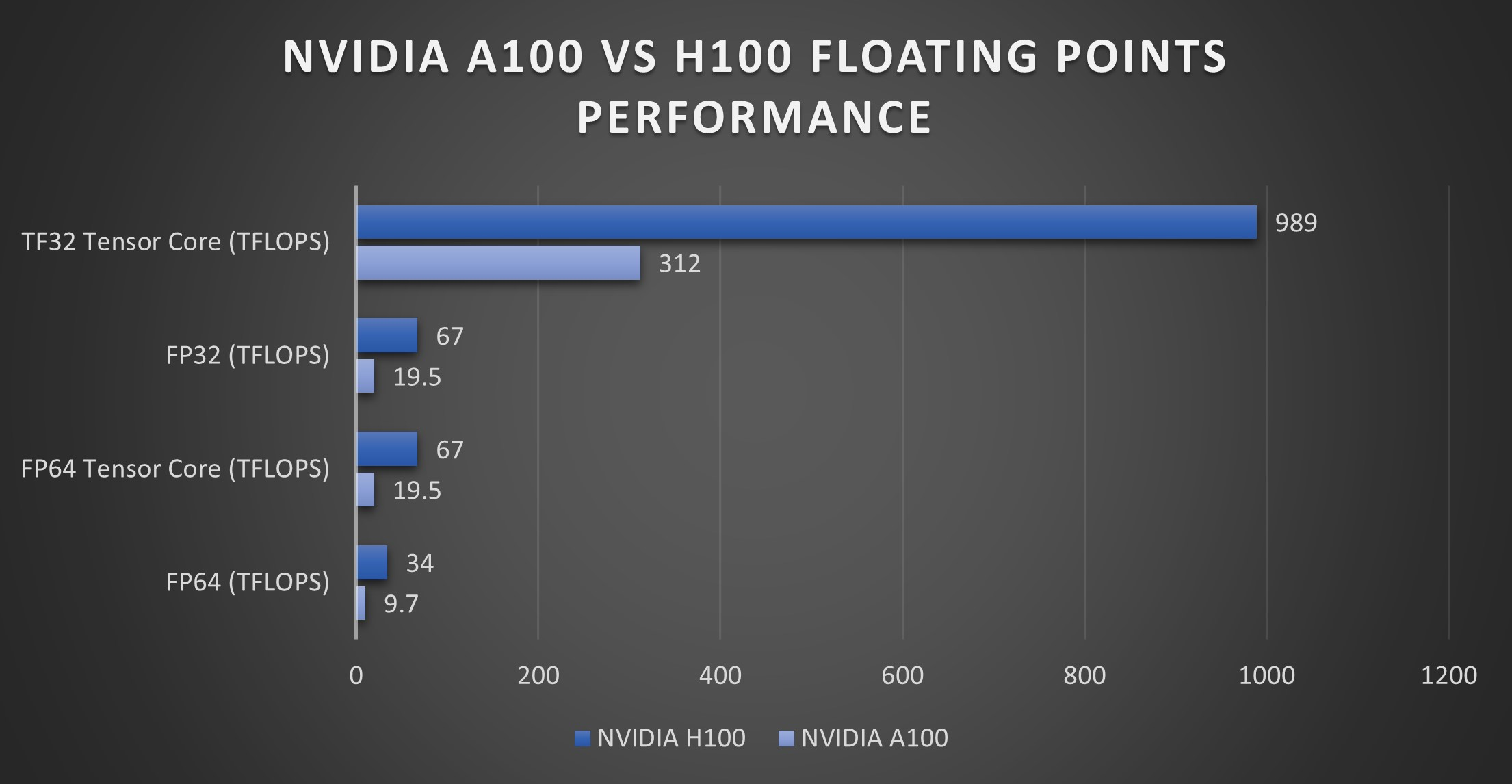
GPUs on Steroids: Tensor Cores (2017). If there was any concern about whether vectorized CPU operations could compete with GPUs, you can throw that all out the window due to the introduction of Tensor Cores with the release of the Volta microarchitecture in 2017. Tensor cores are specialized hardware units for performing 4×4 floating point matrix multiplications extremely fastCertain smaller precision data types like FP16 and FP8 are faster on later editions of Tensor Cores.. Because matrix multiplication can be re-written as block matrix multiplication and deep learning consists of a small set of operations, Tensor Cores are extremely useful, and optimizing throughput often comes down to sufficiently feeding the Tensor Cores. See Figure 14 for a comparison of Tensor Core speed on A100/H100 GPUs.

Intra-Device Bandwidth: PCIe vs. SXM & NVLink. When dealing with larger workloads, another bottleneck to consider is device-device and host-device communication bottlenecks. The standard interface is Peripheral Component Interconnect Express (PCIe), which can be used to connect devices to other devices or to the host. PCIe lanes connect your devices, and a larger number of lines provides more (potential) throughput for data movement. Starting from the Pascal microarchitecture, NVIDIA also began selling GPUs with the SXM form factor, which basically means they have specific ports for SXM interconnects and are connected on a specific SXM board (it still communicates to the CPU through PCIe). The SXM GPUs can also use NVLink, which is a special protocol for larger memory bandwidth. Generally, unless you are dealing with huge workloads, the type of intra-device communication will not even be the bottleneck you are looking for. For example, the H100 PCIe device-to-device bandwidth is 2 TB/s, while the H100 SXM5 device-to-device bandwidth is 3.35 TB/s.

Other relevant optimization details you can just assume exist. Understanding how to use these often involves profiling kernels and balancing the limited amount of “fast” memory we have. Many of these optimizations are highlighted in this amazing article on optimizing matrix multiplication in raw CUDA: https://siboehm.com/articles/22/CUDA-MMM. Because our GPU compilers aren’t unbeatable, it is useful to know many of the following details:

• Shared memory: I didn’t mention this explicitly in the memory hierarchy above, but shared memoryNot to be confused with OS shared memory. The naming here is kind of confusing I’ll admit… is SRAM that is shared between all threads in a thread block. Many tricks involve using shared memory accesses over HBM accesses.
• Thread coarsening: There is overhead for launching threads (it’s not free!) so sometimes it’s actually better to perform sequential operations on the same thread.
• Memory coalescing: When we access HBM/DRAM, it is faster to access them in “bursts”, or contiguous chunks. In other words, we like structured accesses.
• Constant memory: A small, global read-only memory that is useful when we have to re-use the same data a lot.
• Pinned memory: When transferring between CPU RAM and GPU DRAM, NVIDIA GPUs have a Direct Memory Access (DMA) unit that handles the memory transfer to free up compute. Because the DMA uses physical addresses, the OS paging system can accidentally cause the DMA to transfer the wrong CPU memory — pinned memory is a primitive to ensure a chunk of memory will not be paged out, giving up speed-ups on this transfer.
• Streams: We can avoid “waiting” sequentially for independent blocking operations by telling the device to put them on different streams, so it is safe to run them concurrently.

Parallel patterns. It is also important to understand what types of operations are known to be parallelizable. In deep learning, we understand that matrix multiplications (matmuls) are extremely efficient, but many other operations are also parallelizable and have well-known design patterns:

• All BLAS operations
• Convolutions
• Stencil operations
• Reductions (e.g. torch.sum())
• Radix Sort
• Merge (e.g. Kogge-Stone and Brent-Kung, useful for state-space models)
• Histograms

A comparison of notable GPU specs over the years. We’ll be using PCIe and not SXM numbers for reference here.

Energy costs. The power consumption of these devices is pretty important to know if you are using your own machines / clusters. I don’t have a strong intuition for these numbers, but generally they float around the $O(100)$ watts range for current high-end GPUs. For example, the A100 80GB consumes 250W when fully utilized, so it would come out to 600 kWh a day, which is roughly 40 USD in electricity bills if you live in the US. Tim Dettmers has a useful blog that explains these power considerations when building your own machine.

II.x.2: Google’s Tensor Processing Units (TPUs)

The CUDA ecosystem is not the only choice for parallel processing. Google’s in-house Tensor Processing Units (TPUs), first introduced publicly in 2016, are a custom application-specific integrated circuit (ASIC) designed for deep learning workloads at Google. TensorFlow and Jax have dedicated compilers for TPUs, making them the standard choice for programming these devices (PyTorch support has been added, but it’s not great).

• While NVIDIA and AMD GPUs have features like the texture cache that are designed for gaming applications, TPUs specialize in high-throughput, low-precision matrix multiplication with low energy usage.
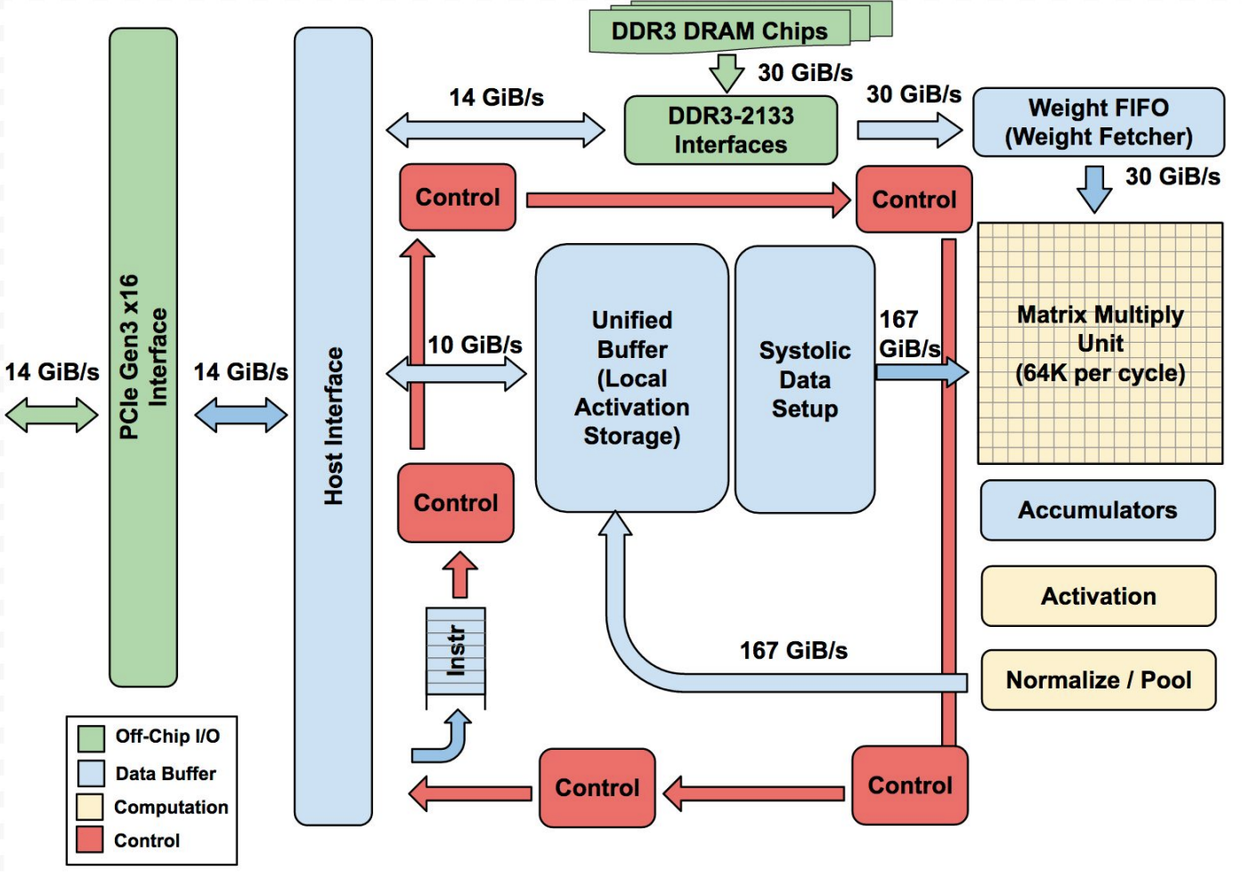
• TPUs use their own systolic array “Tensor Core”, which handles 128×128 multiply-accumulate operations (compared to the 4×4 for NVIDIA!) in a single instruction cycle. This design favors large matrix computations.
• The TPU features special instructions and hardware for activation functions and a super-fast buffer for moving data.
• Google has since come out 6 generations of TPUs, with the latest using 256×256 Tensor Cores to accelerate even larger model computations.
• You can’t actually buy your own TPUs, and you have to use cloud-provided TPUs (or work at Google) to use them for your own applications.
• Similar to the design of SXM boards for NVIDIA GPUs, TPUs also have dedicated “TPU Pods” to connect multiple devices with high-speed communication.

II.x.3: Potpourri of other interesting hardware

The popularity of NVIDIA GPUs is in part due to the success of the Transformer and other parallelizable architectures. However, for different memory access patterns, there exist other hardware alternatives that could later play a pivotal role in the field.

Field-gate Programmable Arrays (FPGA). FPGAs have seen some use in efficient deep learning as a low-cost hardware to target. Because of the availability of GPUs and ASICs like TPUs, it is hard to justify designing and programming these devices for actual workloads. Nevertheless, I wouldn’t write off FPGAs — they have a variety of use-cases in the sciences and low-latency applications, and there is a chance that they will become important in deep learning as well.

Neuromorphic Chips. We know that the human brain is extraordinarily efficient and powerful (except maybe mine), so a natural question is whether we can design computer hardware around the brain. There are some primitives like Spiking Neural Networks that have been designed in the past, but most of this work has not really taken off in “modern deep learning”. There are also some small neuromorphic chips like IBM’s TrueNorth, but I haven’t seen significant progress in this area yet. Like quantum computers, however, I am hopeful that people crack this research direction and apply them to AI!

Etched (2024) [site]. Very recently, a startup company came out with a Transformer-specific ASIC called Sohu that they claim accelerates Transformer workloads (not sure if it’s also training?) by an undefined margin. Little information is known about the underlying hardware and how good it actually is, but a Transformer-specific ASIC itself is not a far-fetched idea.

Part III: The Era of Scale till we Fail (2020-Now)

GPT-3 (OpenAI, 2020). The introduction of GPT-3 was eye-opening for a lot of researchers in the field — simply scaling a Transformer to 175B parameters while maintaining the same tricks used in prior works in the field was sufficient to build a syntactically sound and somewhat semantically reasonable model. Furthermore, while most prior works had been task-specific, GPT-3 was flexible enough to perform reasonably on a wide variety of language tasks.

Its successor, GPT-3.5 / ChatGPT would later blow up the field of AI to the public, but these methods would introduce a combination of new post-training tricks (instruction-tuning & RLHF) and better data that are not rigorously understood. Scaling these models became a whole new game than all previous works, with the goal of building general-purpose “foundation models” that could be applied to any task. For this reason, the rest of this post will primarily focus on transformer-based architectures or recent alternatives (e.g. state-space models, Kolmogorov-Arnold Networks). Many of the following ideas certainly apply to existing deep learning methods, and molding these approaches to older algorithms is definitely a useful research direction that may yield meaningful results.

Part III.0: Let’s talk about the H100 GPU

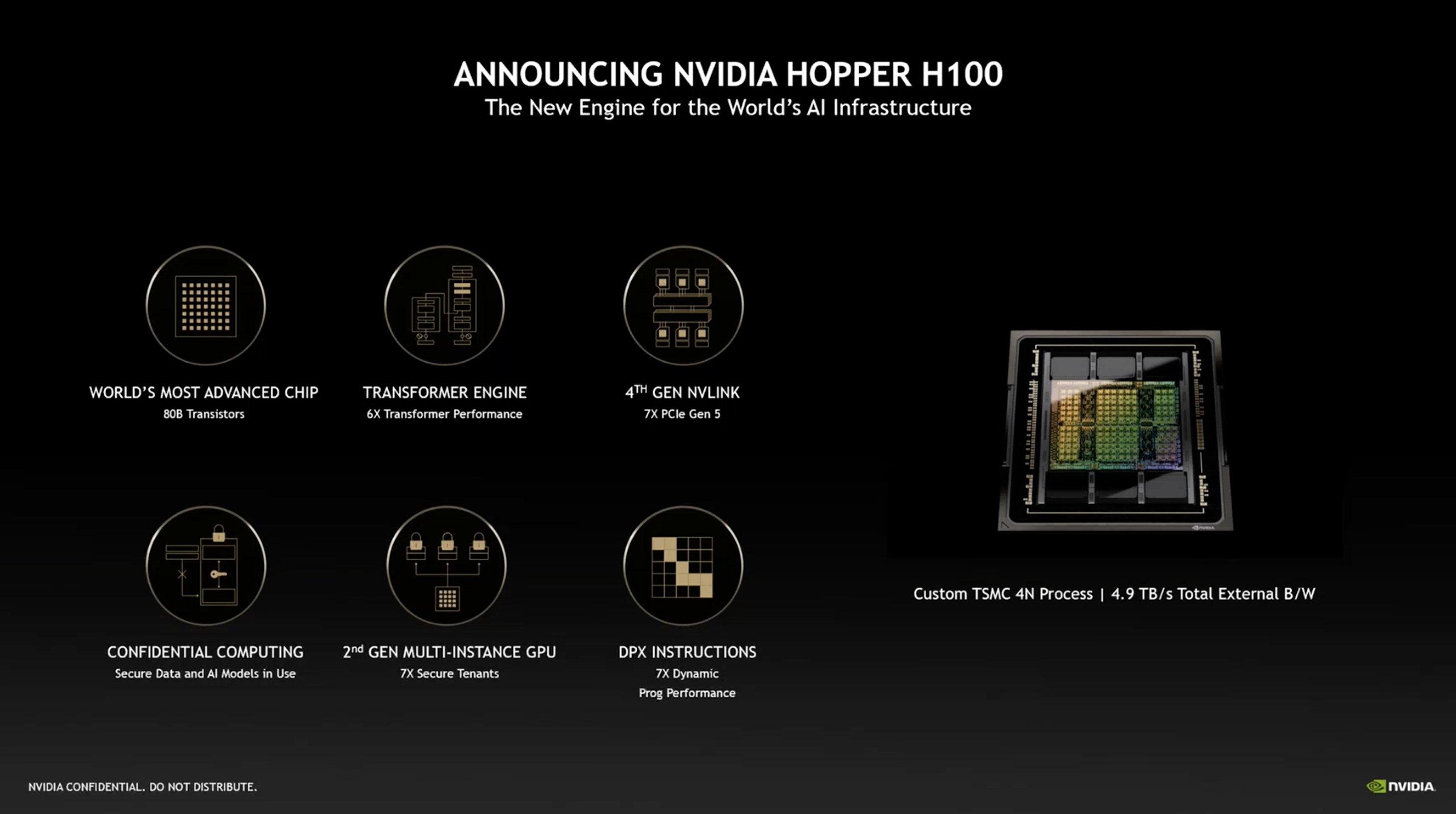
NVIDIA’s Hopwell microarchitecture (2022), along with the H100/H200 GPUs, introduced a few notable new features to accelerate deep learning workloads. In addition to having effectively more/faster memory, higher memory bandwidth, and more CUDA & Tensor Cores than the A100, the H100 also features:

• Tensor Memory Accelerator (TMA). The whole concept behind “streams” that we introduced before was to ensure non-overlapping operations like memory movement and using the Tensor Cores were done in parallel. The TMA is a new hardware unit that asynchronously computes memory addresses (this is not a free operation on older devices and had to be done with registers!) for fetching data between shared memory and global memory. In other words, we no longer need to dedicate threads to perform data transfers and can instead focus on feeding the Tensor Cores.
• High-speed low-precision. Tensor Cores now support the FP8 data type and can theoretically reach 3300 TFLOPS for FP8 operations.
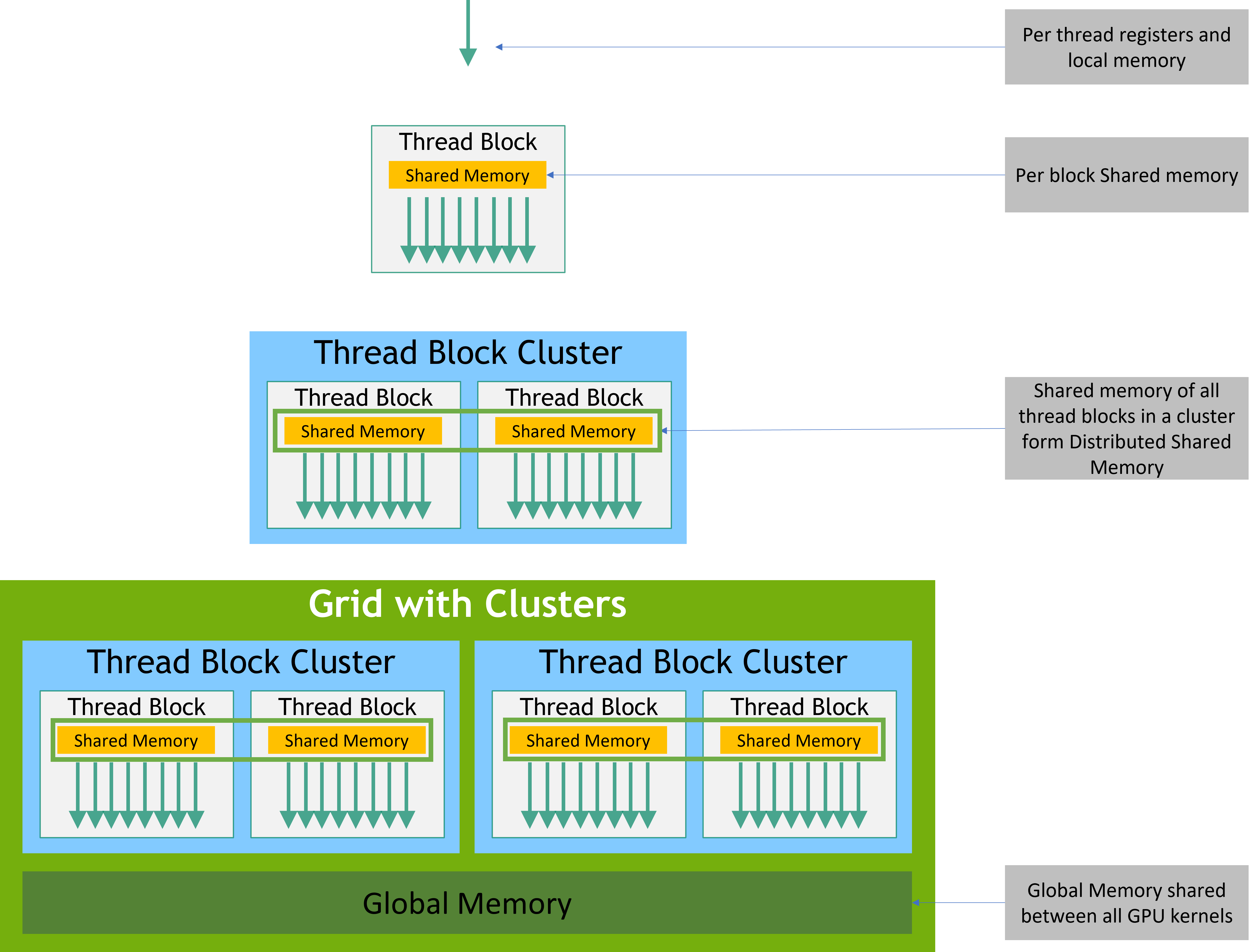
• Thread block clusters. A new level of the CUDA programming hierarchy sits above the thread block — all threads in a thread block cluster are concurrently scheduled onto SMs, making communicating between them more efficient with the CUDA cooperative_groups API.
• SM-to-SM shared memory. They formally call this distributed shared memory, but basically a programmer can now access shared memory that sits on other SMs (presumably through a shared virtual address space) without having to move it to the L2 cache / global memory.
• DPX instructions. The promotional material for these instructions keeps claiming that they “accelerate dynamic programming (DP) algorithms”, but I’m pretty sure from the Hopper guide that it’s just specialized instructions for min/max and additions that are common in DP algorithms — the actual loop and sequential nature of DP isn’t changed at all.

With the release of the H100, a few interesting developments have been made to target these devices, including FlashAttention3, which we will talk about in the coming section.

WGMMA (Warpgroup Matrix-multiply-accumulate)This blogpost by Colfax is so good: https://research.colfax-intl.com/cutlass-tutorial-wgmma-hopper/. The wgmma.mma_async instruction allows threads to launch matrix multiplication on the Tensor Cores as a non-blocking operation. In other words, they’re free to handle other tasks like data loading to further increase throughput and hide latency.

ThunderKittens (Spector et al., 2024). The H100 has a lot of new features that are really annoying to target yourself. ThunderKittens is a domain-specific language (just an extension on top of CUDA C++ basically) that you can use to abstract away a lot of these features at the warp-level while the compiler handles all of the nitty-gritty details. I haven’t tried it myself because I don’t have an H100, but it looks like a promising library to consider using. I also included the blog in this section because it has some nice details about how they target the H100 that are really well-written!

Part III.1: The Era of Scale (on a single GPU)

By this point, there were clear signs that scaling up the number of parameters in a model and the amount of data was almost purely beneficial for improving model capabilities. The obvious solution to scaling networks was to 1) add more compute and 2) wait for longer training runs. But adding devices is extremely expensive and does not linearly add more memory and training speed as we will discuss in Part III.2, so there was a lot of interest in squeezing out as many FLOPS and bytes out of every GPU as possible. Before it was settled that the attention mechanism was extremely important as is, alternatives with better runtime and memory scaling were first proposed.

III.1.0: Early insights

Activation checkpointing (Chen et al., 2016). One widely used technique for trading speed for memory is to re-compute activations during the backwards pass instead of storing them during the forward pass. This idea is also used to speed up overall training in important works like ZeRO due to the nature of the GPU memory hierarchy, which we will cover in the next section.

KV Caching (2017?).I actually have no idea when this trick was first introduced — my guess is that it was sort of an obvious engineering trick that people knew about for a while, but didn’t really need to talk about in publications until LLM serving became bigger as a field / after ChatGPT came out in 2022. For causal Transformers (upper-triangular mask), a well-known trick for next-token prediction is to store the previously computed keys and values in memory, so we only need to compute $K/V/Q $ for the most-recent token. A large number of works we will discuss deal with the growing KV cache, which takes up a large chunk of valuable DRAM and is not a fixed size.

III.1.a: Shaving complexity through Approximate Methods

A long series of works have proposed approximations to the general attention mechanism in hopes of scaling these methods to sub-quadratic memory and runtime. We list some notable examples in chronological orderNot all of the code examples are the official code repos. I referenced lucidrains a lot because his (PyTorch usually) repos are just a lot easier to digest and are stripped down to the important code.:

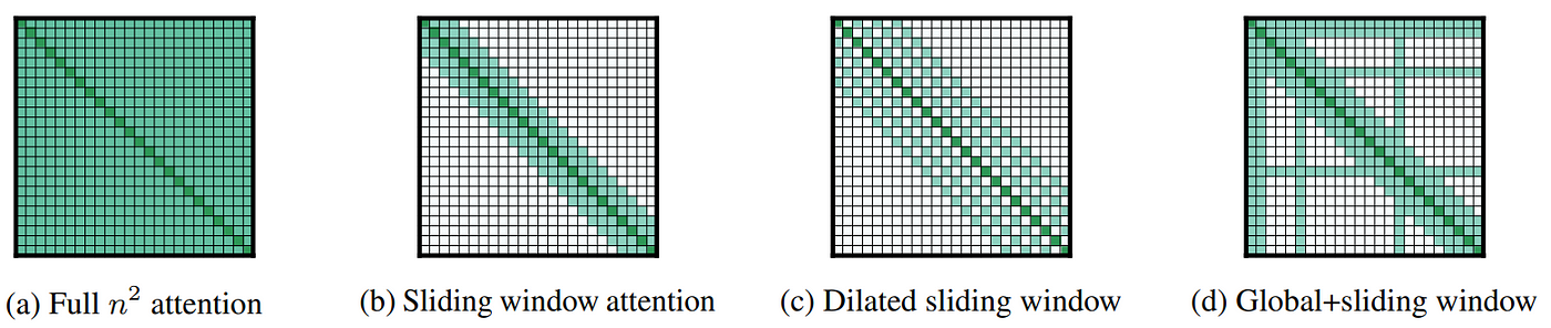
• Sparse Transformers (Child et al., 2019) [Paper] [Code]. Early work on constraining fixed sparse attention patterns (across heads, though this isn’t too relevant anymore) so each query can only attend to $O(sqrt{N})$ of the keys. They evaluate on a variety of image and audio tasks, although the results aren’t high quality for today’s standards.
• Reformer (Kitaev et al., 2020) [Paper] [Unofficial Code] This idea is really cute — they posit that attention weights are largely concentrated on a few elements, so they use a locality-sensitive hashing scheme find the $K=log(N)$ nearest keys for each query and only compute those for the attention mechanism.
• Linformer (Wang et al., 2020) [Paper] [Unofficial Code]. They reason using the Johnson-Lindenstrauss lemmaThere are many variants, but the core idea is that we can (randomly) project points in a high-dimensional normed space to a lower-dimensional normed space such that distances are preserved up to some error that is a function of the number of points in the space. Basically, it’s used a lot whenever we want to analyze whether moving to lower dimensions is “fine”. that when computing the attention matrix, they actually just compute it as a product of two low-rank matrices. Their proposed decomposition is extremely simple, and it literally is just projecting down the key and value matrices to a constant dimension.
• Longformer (Beltagy et al. 2020) [Paper] [Code]. Longformer is just an empirically-motivated set of masking patterns over the attention matrix for efficiency. They mainly use a sliding window local attention scheme (see Figure 17), but also allow attending sparsely to global positions.
• Performer (Choromanski et al., 2021) [Paper] [Unofficial Code]. Instead of using a low-rank or sparsity assumption, they observe that the attention operation $A(i,j) = exp(q_i, k_j^T) = K(q_i, k_i)$ is a kernel, which can be written in the form $phi(q_i)^T phi(k_i)$. The choice of $phi$ is motivated to be an unbiased estimator using random featuresSee https://gregorygundersen.com/blog/2019/12/23/random-fourier-features/ for background., and ultimately the decomposition removes the annoying softmax function and reduces the number of operations.
• InfiniAttention (Munkhdalai et al. 2024) [Paper] [Unofficial Code]. InfiniAttention avoids sequence-length time/memory complexity by storing a recurrent-style attention matrix that is fixed size, but is updated in memory. They chunk up sequences and sequentially process them, theoretically enabling infinite scaling at the cost of a fixed representation.

While many tricks like sparsity, low-rankness, and kernel decomposition were tried, in the end, most of these methods are unused in modern LLMs. Some of the more practical approximations for the attention mechanism are a lot simpler in practice and provide clear memory or runtime improvements over the original.

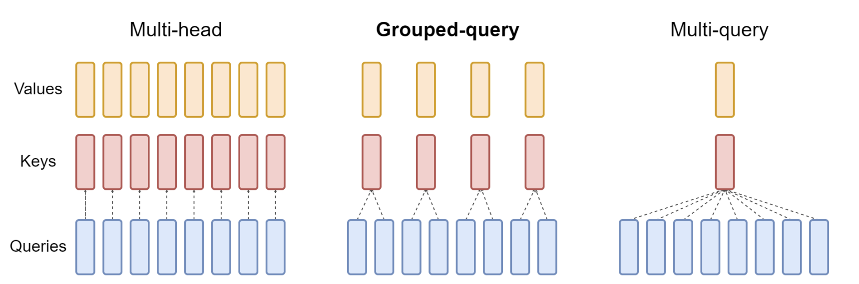
Grouped Query Attention (Ainslie et al., 2023). A super simple but widely used approximate attention method is to preserve the standard per-head attention, but instead share keys/values across different heads to reduce the memory footprint. The original work (multi-query attention) re-used the same keys/values across all heads, but in this work they find it better to tune this re-use factor. It turns out that we can get away with this in practice, and from an implementation stand-point there is no hidden drawback to doing this.

III.1.b: Architecture Design

Some architecture choices have been motivated by existing bottlenecks in scaling large models. For language models, the naive approach is to just increase the number of attention blocks, but there are other methods that balance memory and capacity tradeoffs differently.

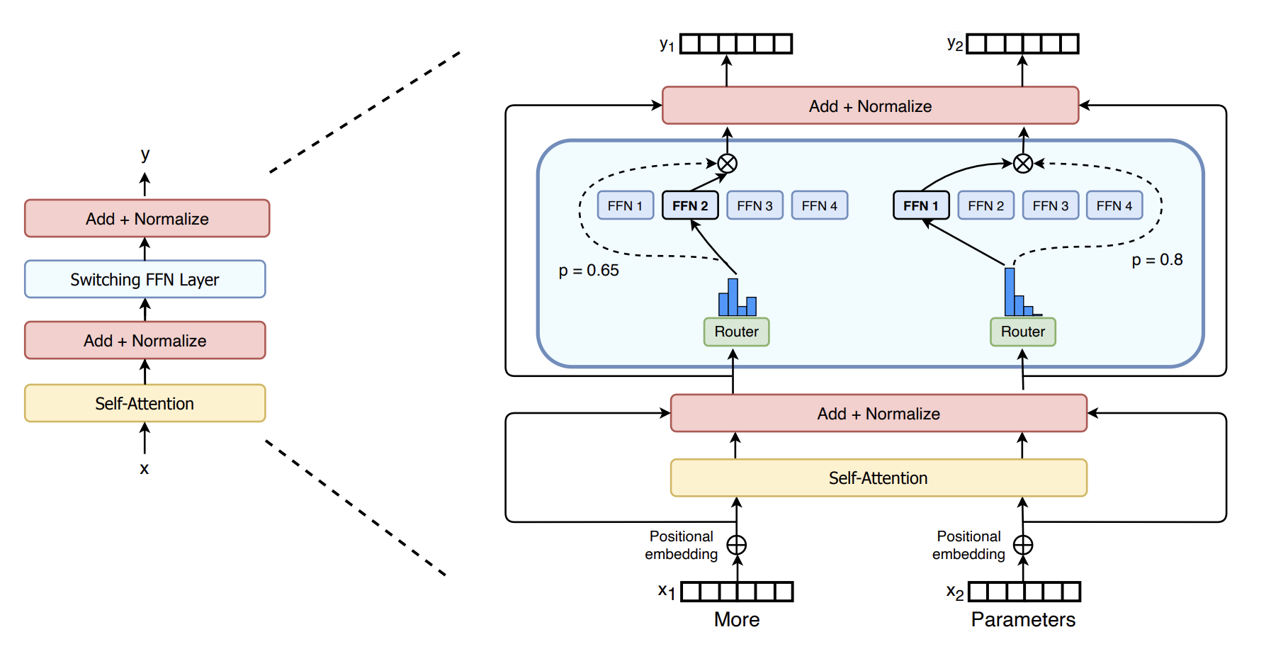
Mixture-of-Experts in NLP (Shazeer et al. 2017). Mixture-of-Experts (MoE) is an older techniqueHuggingface has a nice article on the history, which dates back to the 90’s: https://huggingface.co/blog/moe#a-brief-history-of-moes for scaling deep learning models to extremely high parameter counts without needing to access all the parameters at any time. The first interesting application was done on the LSTM architecture, and generally it consists of a small learnable gating network that activates a subset of the parameters sitting on different devices. As we will see, MoE is particularly useful for LLMs, as it enables scaling model capacity without scaling the resource consumption.

Primer: Searching for Efficient Transformers for Language Modeling (So et al., 2021). There are plenty of existing works for tweaking and modifying the attention architecture to “scale” better. I’ve referenced this paper because it is quite simple and is one of the earlier works to propose tricks like ReLU^2 and neural architecture search over Transformers. I’m not entirely sure what is done in practice, but as far as I know, there are generally some “good practices” for Transformer blocks, and it is difficult to perform these architecture search algorithms for extremely large models.

Switch Transformers (Fedus et al., 2021). Their central hypothesis was that scaling model parameters while keeping FLOPS constant was still a useful dimension of scale. They replace the FFN MLP layer in the Transformer with an MoE router that routes each token after the attention block to an expert, while also fixing the maximum number of tokens each expert can process. They also add a super simple load-balancing loss that penalizes non-uniform token routing. As it turns out, MoE enables us to scale our models to upwards of trillions of parameters without actually incurring the cost of a trillion parameter model on each forward/backwards pass! It was rumored last year that GPT-4 was a giant 1T MoE model that used tricks like group-query attention and rotary embeddings (RoPE).

III.1.c: Fine-tuning Large Models Efficiently

It is well known that pre-training large foundation models is way out of the budget of a standard researcherFor example, Llama-3 is known to have cost tens of millions of dollars to pre-train.. Fine-tuning or general post-training (e.g. instruction tuning and RLHF) has become a popular research avenue because it is significantly cheaper and can be task-specific. Researchers began to notice over time that shortcuts could be made to the fine-tuning process to make it feasible for independent researchers to play with.

Adapters (Houlsby, 2019). The distinction between fine-tuning and pre-training is actually indistinguishable from a standard machine learning perspective, unless we specifically constrain the optimization problems to be different. To make fine-tuning computationally cheap, Adapters are learnable functions $f_{hat{theta}} : mathbb{R}^n rightarrow mathbb{R}^n$ that can be inserted in between the layers of a model. The idea is that we freeze the original model weights $theta$, and only update the adapter weights $hat{theta}$, significantly reducing the memory and fine-tuning time of a model. Intuitively, adapters make sense in the context of language modeling because we believe that fine-tuning should not alter the weights “that much””that much” is super hand-wavy. I’m not actually sure if there’s a paper out there that uses norms or other metrics to discuss similarity between a fine-tuned and pre-trained model. If not, could be an interesting research question. from the base model.

LoRA (Hu et al., 2021). Given a pre-trained model with parameters $theta$, the central hypothesis of LoRA is that a fine-tuned model weights can be decomposed into $theta + Delta hat{theta}$, where $Delta hat{theta} in mathbb{R}^{m times n}$ is low-rank and $theta$ is frozen. In other words, we can factorize $Delta hat{theta} = AB$ where $A in mathbb{R}^{m times r}$ and $B in mathbb{R}^{r times n}$ and $r ll min(m,n)$Strangely, I don’t have a lot of intuition for learned matrix decomposition. This idea is popular in recommendation systems / factorization machines, and is supposedly SVD-esque, but I don’t know what properties you can derive from these factorized matrices. If anyone knows, please tell me! . Furthermore, unlike adaptors, LoRA adds no extra overhead during inference time!

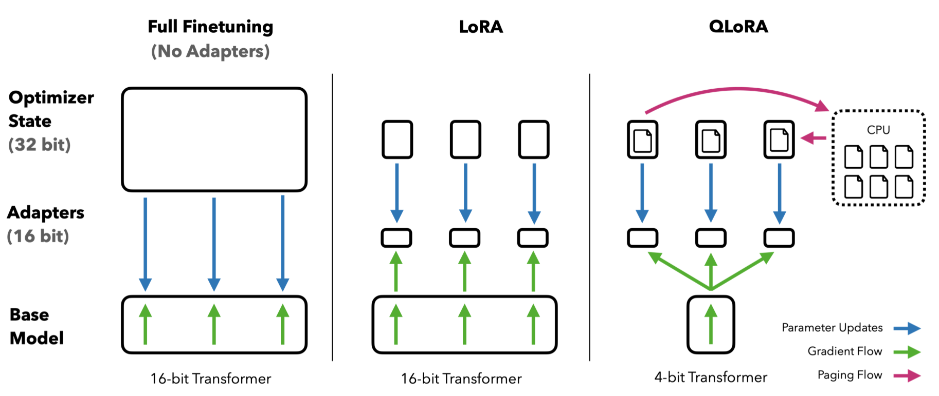
Q-LoRA (Dettmers et al., 2023). This landmark paper enabled a lot of future work on fine-tuning LLMs, diffusion models, and other foundation models on a single device. They observe that 1) base models are still huge and need to fit in memory when using LoRA, 2) activations/gradients have a large memory footprint in LoRA, which activation/gradient checkpointing can partially solve, and 3) block-wise quantization can have many constants take up significant space in memory.

• To solve (1), they introduce the 4-bit NormalFloat type, which quantizes the weights by evenly dividing the range based on the Gaussian measure.
• To solve (2), they introduced a paged optimizer based on NVIDIA unified memory to move optimizer states between GPU DRAM and CPU RAM when necessary, as they are only used for backpropagation.
• To solve (3), they quantize the quantization constants to a lower precision. Q-LoRA is basically a whole collection of memory reduction techniques for performing LLM fine-tuning on affordable hardware. The LoRA component remains untouched, but the memory reductions allow LoRA to be applied to all layers in a model for better performance.

Combined together, a Q-LoRA tuned layer can be written as:

$$
f(X^{(bf16)}) = X^{(bf16)}text{dequant}(W^{(NF4)}) + X^{(bf16)}A^{(bf16)}B^{(bf16)}
$$

Huggingface PEFT Library. There are a few other major parameter-efficient fine-tuning (PEFT) works like LoRA and adaptors such as prefix tuning, soft prompts, and $(IA)^3$ that all kind of boil down to “I believe that we can fine-tune a model by slightly adding or injecting information to the pre-trained model”. Honestly, PEFT as a whole is extremely hand-wavy, and a lot of the methods are ways to condition or perturb model weights based on the fine-tuning dataset. HuggingFace has a nice wrapper for running different PEFT methods for your models. For details on specific PEFT variants, I’d suggest reading this survey paper.

Remark. I couldn’t really fit this work in, but I wanted to mention ReFT, which I think is a really cute idea that turns out to work well in practice. Based on the hypothesis that high-level concepts in language model are directions in some representation space, they fine-tune model generations by learning disjoint “interventions” over the model hidden states (i.e. an adapter motivated by interpretability work). I haven’t fully read into the interpretability work that led to DII, but their experiments are pretty convincing.

III.1.d: Fused kernels and the GPGPU

Read Part II.x: Hardware before continuing in this section.

Eventually, it became clear that cute tricks like sparsity and dimensionality reduction on the attention mechanism were not only hurting model performance, but they weren’t even providing wall-clock speed improvements to these models. You may have heard the term “fused kernel” used to describe an optimization to a deep learning model. The term kernel is overloaded quite often, but in this instance it just refers to a program run on the GPU. We focused a lot in the earlier sections on building up models as modular, stackable components that we could freely optimize, but allowing this flexibility is not necessarily hardware-friendly. Consider the following example for computing the attention operation in PyTorch:

$$
mathbf{O} = text{softmax}left( frac{mathbf{Q} mathbf{K}^T}{sqrt{d_k}} right) mathbf{V}
$$

def attention(Q: torch.Tensor, K: torch.Tensor, V: torch.Tensor) -> torch.Tensor:
d_k = math.sqrt(Q.size(-1))
scores = torch.matmul(Q, K.transpose(-2, -1)) / d_k
p_attn = scores.softmax(dim=-1)
O = torch.matmul(p_attn, V)
return O

In eager execution mode or without a clever compiler, every assignment $y = f(x_1,x_2,…)$ in the code above will do something like this.

1. The variable(s) $x_1,x_2,…$ will be sitting in the GPU DRAM/HBM. We first have to load it onto the processors/SMs, which is quite slow.
2. We perform the transform $f(x_1,x_2,…)$ on device. This operation is relatively fast because the torch functions (e.g. torch.matmul) are heavily optimized.
3. We store the result $f(x_1,x_2,…)$ which sits on device registers back into DRAM, and point to it with the variable $y$.
4. If $y$ is ever used in subsequent lines, we have to load it back into registers, and repeat.

Fused kernel implementations usually aim to remove these intermediate stores and loads to DRAM that Python compilers cannot optimize out. Depending on the level of granularity in the language used (e.g. Triton vs. CUDA), we can control data movement at all levels of the GPU memory hierarchy. To get a sense for the relative speeds of each level of the hierarchy, we list some data movement speeds on an NVIDIA H100 GPU found in this microbenchmarking work. For reference, the H100 runs at roughly 1.5 GHz, or $1.5 times 10^9$ clock cycles per second.

In the following section, we’ll talk a bit about existing fused kernel strategies for attention, followed by some examples in other fields.

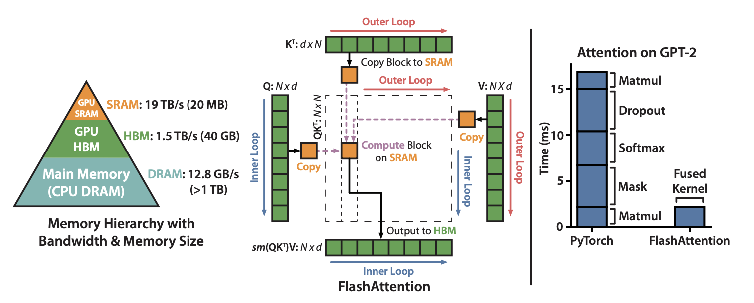
FlashAttention (Dao et al., 2022). Standard attention implementations, like the PyTorch implementation above, involve several passes to and from GPU DRAM/HBM. The key insight in building the fused attention kernel is computing the softmax block-by-block — however, computing the softmax requires loading all keys into a block, which does not fit into the limited SRAM space. The authors instead minimize accesses to global memory by using a trick called the online softmax while simultaneously loading in the relevant value blocks. Furthermore, they re-compute the attention matrix in the backwards pass. Launched kernels are parallelized over the batch size and the number of heads.

FlashAttention2 (Dao, 2023). The successor implementation of FlashAttention minimizes non-matrix multiplication operations such as the online softmax scaling term, which are significantly slower due to A100 Tensor Cores — while the max throughput for FP16 matmuls is 312 TFLOPS, for standard FP32 operations it is only 19.5 TFLOPS. Furthermore, they avoid intra-warp synchronizationRecall that threads in a warp call the same instructions SIMT-style. However, across warps in the same block, we often will call a block-level synchronization barrier with `__syncthread()` when we need to wait for all previous threads to finish. The authors minimizes these barrier calls in FA2 by changing which warps handle which matrices. If this whole explanation is confusing to you, I totally understand. The original paper has some nice diagrams that explain it better, but it’s definitely a GPU-specific detail. by switching how they loop over the $mathbf{Q}$ and $mathbf{K}/mathbf{V}$ matrices. One particular limitation of these methods is no support for custom attention masks and attention biases, which is now supported in FlexAttention as of August 2024 (I also had written a Triton implementation for FA2).

FlashAttention3 (Shah et al., 2024). The latest version of FlashAttention specifically targets the H100/H200 GPUs, and the focus reads completely differently from v1 and v2. Namely, the new WGMMA instruction we talked about in Part III.0 and the TMA offer essentially free speed-ups. Furthermore, separating data loading (TMA) and computation (WGMMA) in different warps, a technique called warp specialization, is also used to maximize Tensor Core usage. Finally, the authors observe that non-matmul operations like exponentiation in softmax are up to 256x slower than matmuls, so they manually schedule warpgroups in a pipelined fashion to reduce potential bubbles created by these interleaved operations.

xFormers (Facebook Research, 2021) [Repo]. The xFormers repository features a series of CUDA and Triton kernels for various Transformer components like attention, layer norms, dropout, etc. Prior to the release of FlexAttention, the xFormers repo was also the standard for a fast attention algorithm with custom attention biases.

Liger Kernel (Hsu et al., 2024) [Repo]. Recently, a large number of fused kernel implementations for LLM training were released by researchers at Linkedin. In addition to being more memory-efficient and faster than pre-existing Huggingface implementations, they are extremely easy to understand because they were written in Triton.Some of these kernels were featured in depth in one of the GPU Mode lectures: https://www.youtube.com/watch?v=gWble4FreV4&ab_channel=GPUMODE

Other examples. While fused kernels have seen extensive interest in transformer-based LLM applications, there are other areas where fused kernels were critical to their success. We list a few notable examples below.

• FlashFFTConv (Fu et al. 2023). It is well known that for functions $u(x), v(x)$ with Fourier transforms $mathcal{F}(u), mathcal{F}(v)$, the convolution can be written as $ {u * v } (x) = mathcal{F}^{-1} {mathcal{F}(u) cdot mathcal{F}(v) } $. It is also well known that the Fast Fourier Transform can be computed in $O(N log N)$, so we can compute convolutions for state-space models in $O(N log N)$ where $N$ is the sequence length! However, despite the better runtime complexity than attention, in practice, Transformers are still faster to train on modern hardware. FlashFFTConv re-writes the FFT into a different decomposition that contains matrix multiplications to take advantage of Tensor Cores.
• Mamba: Linear-Time Sequence Modeling with Selective State Spaces (Gu et al., 2023). Prior state-space model methods (e.g. S4) impose a linear-time-invariant (LTI) constraint on the state update matrices so they can be re-written as a convolution to avoid the sequential computation needed for recurrent algorithms. While these models were interesting at the time, Mamba was a huge deal in the community because it removed the LTI constraint and added an input-dependent selection mechanism for its parameters. To remove the LTI constraint, the authors wrote a kernel to keep the recurrent state in fast shared memory to keep the computation fast.
• InstantNGP (Müller et al. 2022). The novel view synthesis problemThe novel view synthesis problem is generating unseen views of a scene given a few reference images. With a fine granularity, you can even produce entire videos or interactable scenes from just an image. has mostly been solved using Neural Radiance Fields (NeRFs), but the computational bottleneck of increasing resolution was large. InstantNGP was a hashing scheme for position-dependent features that was entirely written as a fused kernel, and is widely used as a standard in many subsequent NeRF works as well.
• MSA Pair Weighted Averaging for AlphaFold3 (Me!). AlphaFold3 is a closed-source scientific breakthrough (most notably winning the 2024 Nobel Prize in Chemistry!) developed by Google DeepMind for predicting generic molecule interactions. While they most likely developed the model in Jax and optimized it for their in-house TPUs, researchers and start-ups outside of Google are interested in using the model for their own biotech use-cases. Ligo Biosciences is a start-up developing an open-source version of this model, but certain algorithms such as the Triangular Multiplicative Update and the MSA Pair Weighted Averaging algorithm have extreme memory bottlenecks when written naively in PyTorch. I was interested in was writing fast and readable kernels for these algorithms (both forward and backwards passes), which I wrote in TritonTriton is a programming language (it’s more of a library for Python) that compiles to an intermediate representation (IR) that NVIDIA GPUs can use. Rather than abstract at the thread-level like we’ve discussed for CUDA, it instead operates at the thread block level, and is far easier to prototype with. We will talk about this later, but torch.jit() compiles to Triton code.. The MSA Pair Weighted Averaging algorithm in particular also has a pesky global softmax operation, and I used tricks similar to FlashAttention2 to minimize HBM accesses. Removing these bottlenecks has helped them feasibly scale their models on more data!

III.1.e: Deep Learning Compilers

Another parallel thread that the community was interested in was building specialized compilersI’m going to assume the reader is at least familiar with what a compiler is useful for. A lot of the optimizations done by programming language compilers like constant folding and register assignment are also done by a deep learning compiler, and LLVM itself is used in this setting for compiling to the instruction-level. for deep learning operations. ML compilers are really annoying to build because 1) there are so many different hardware devices that we can use (e.g. CPU, GPU, TPU, other ASICs), 2) in a standard compiler like gcc, we would normally have access to the entire codebase we are compiling. For ML, a “codebase” is basically the model computation graph, but this isn’t always accessible (i.e. eager mode in PyTorch)On point (2), you probably don’t need a powerful compiler unless you are running production code, in which case you should not be running your models in eager mode. Regardless, as we will see, the PyTorch team still added an option through torch.jit() for compiling parts of your eager execution code..

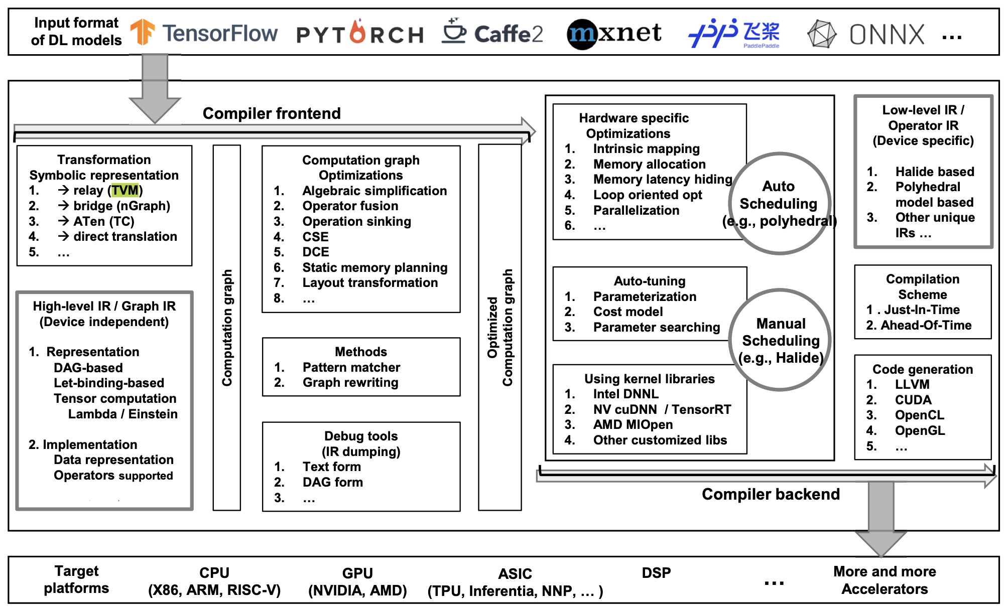
Intermediate representations (IR) are a critical element of modern compilers — instead of building a compiler for each pair of (language, hardware), we would ideally like to compile each language into a common intermediate language that can be converted to each specific machine code. Deep learning applications are typically optimized in two steps, namely graph-level optimization of operators, and low-level optimization of the actual device-specific instructions. Below, we discuss some important frameworks and compilers that have evolved throughout the years — the list is not comprehensive (check out https://github.com/merrymercy/awesome-tensor-compilers!), but focuses mainly on applications that have been popular for a while.As I was researching this section, I came to the realization that a lot of it starts to bleed into standard compilers research, which is extensive and difficult for me to motivate. I’ve instead decided to just provide some high-level intuition for what these frameworks do, but I won’t be touching on the exact optimizations and design choices for each of these compilers, which was my original intention.

ONNX (PyTorch Team, 2017). ONNX is not actually a compiler, but an open-source standard format and inference engine (ONNX Runtime) for model computation graphs across different libraries. Most libraries allow you to export your models to ONNX, allowing you to use their optimized runtime engine, as well as convert models easily between libraries. Many of the libraries listed below accept or expect a packaged ONNX model as input.

Agnostic stacks. These frameworks are designed for developers to be able to modify and add certain parts of their compilers stack (e.g. targeting your own edge devices), and are widely used as general purpose compilers. They often features multiple IR conversion and optimization steps, and provide functionality for targeting your own hardware.

• TVM (Chen et al., 2018). TVM is an open-source end-to-end compiler stack for common deep learning platforms and targets a wide range of hardware. TVM first converts compute graphs into a directed-acyclic graph (DAG) IR called Relay — you may have learned about let-based IRs in your undergraduate compilers class that allow for optimizations like dead-code elimination, and a DAG IR is basically just the equivalent for a graph. The individual tensor operators have a separate optimization step, and TVM uses functional “tensor expressions” to define these operators. TVM has a ton of other really cool features like auto-tuning for specific data/hardware formats that are beyond the scope of what I really understand, but I would highly recommend reading the DL compilers survey for a high-level overview of TVM and other compilers.
• MLIR. The Multi-Level Intermediate Representation (MLIR) is an extension to LLVMAgain, sort of assuming you know what it is. In case you don’t, LLVM is a really powerful and language-independent library that features the LLVM IR. You would generally convert your language of choice into the LLVM IR, LLVM would perform a bunch of optimizations, then it would convert the IR into your hardware of choice. Before LLVM, dealing with compilers across different hardware was a pain in the ass. LLVM is also used for these deep learning compilers as well. that essentially allows you to define your own IR / dialect based on existing MLIR dialects — in other words, you don’t have to define an IR completely from scratch. MLIR is extremely useful in the context of deep learning compilers, because we often care about multiple optimization passes at different abstractions, which MLIR gives you the flexibility to define. MLIR works well with a lot of the compilers / tools we will list below — to get started, I found this post pretty helpful: http://lastweek.io/notes/MLIR/.

Examples of prominent specific-compilers. These compilers are technically general-use, but are mostly used to target specific devices or specific libraries. Unlike the frameworks above, they are highly optimized for specific use-cases and are much more useful as tools rather than personal development. If you’re not very interested in compilers, it is nice to know some of the stuff listed below.

• nvcc (NVIDIA, 2007). nvcc is NVIDIA’s compiler for CUDA to PTX (NVIDIA GPU’s assembly code). As far as I’m aware, a lot of the details about how what the compiler does under the hood are proprietary.
• XLA (Google, 2017). The accelerated linear algebra (XLA) compiler is mainly for linear algebra workloads in TensorFlow/Jax. It also features a just-in-time (JIT) compiler and operates at the computation graph-level. The OpenXLA project designed it to be able to target other non-TPU hardware as well.
• TensorRT (NVIDIA, 2019). TensorRT (and now TensorRT-LLM) are inference engines that target NVIDIA devices. Given a computational graph in PyTorch/Tensorflow or ONNX, these libraries apply a set of optimizations (e.g. layer fusion, quantization, kernel selection) on CUDA devices for low-latency inference.
• PyTorch’s Compilers over the Years. PyTorch supports both eager execution and graph execution, and it compiles these separately. Recently, PyTorch 2.0 introduced the torch.compile() decorator for easily applying JIT compilation to your code (with some restrictions of course). The PyTorch umbrella includes several different compilers such as the two-phase IR Glow (2018), nvFuser (2022), and the JIT compiler TorchDynamo + TorchInductor.
• Triton IR (Philippe Tillet / OpenAI, 2021). Triton is a domain-specific language for programming NVIDIA GPU kernels in PythonIf you’ve used Triton, you’ll notice the compute hierarchy is less granular than CUDA. Kernels operates at the block level, and there are specific functions for loading memory into threads. The other downside is the reliance on the Triton compiler when new hardware comes out, e.g. targeting H100 features like the TMA.. By default, the torch.compile() function generates Triton code using TorchInductor. Triton has its own compiler, which converts Triton code into the MLIR-based Triton IR. The Triton-JIT compiler then optimizes this code and generates PTX code. I have found Sasha Rush’s GPU Puzzles to be quite useful (my solutions). I also found the Liger Kernel repository, which we talked about earlier, to be a well-written set of examples for learning Triton.

Remark. There is honestly a lot more to talk about regarding deep learning compilers, and compilers in general, but it is hard to motivate it at a high-level without going into details. There’s also a lot that goes into the design choices for specific optimizations, and I’m really not an expert on this stuff. I linked this earlier, but I did find The Deep Learning Compiler: A Comprehensive Survey to be extremely informative on the design choices of these compilers.

Part III.2: The Era of Scale (distributed version)

Imagine that you are a {insert big tech company or unicorn startup} in 2020, and you are now a big believer in scale — you want to build, say, a trillion parameter model, but you now have a whole suite of new problems in the distributed setting. I previously mentioned adding more GPUs as an “obvious” solution to scaling models, but doing this is a lot harder than it sounds — a lot of work goes into minimizing various overheads, circumventing communication errors, and building fault-tolerant and stable algorithms for distributed workloads.

III.2.a: Data parallelism

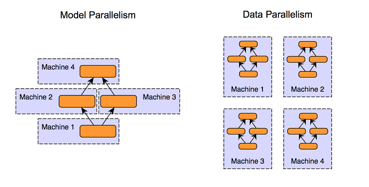
Suppose I have a 1B parameter (~2GB) language model that I want to train on the C4 dataset (~750 GB). One common approach to accelerating training is to increase the batch size to increase the training throughput by taking advantage of the GPU’s parallelism (e.g. Llama 3 uses a batch size of each least 250K). Because we know that models make updates after batches of training, the naive approach is to put a copy of the model on each GPU and distribute the batch across multiple GPUs so it can fit in memory. Certain libraries like PyTorch have wrappers that handle distributing and gathering gradients across GPUs to make sure the model copies on each device are in syncSee the DistributedDataParallel module: https://pytorch.org/docs/stable/generated/torch.nn.parallel.DistributedDataParallel.html. The most common data parallel scheme is to distribute a large batch of samples $B$ across many devices, compute the forward and backwards passes, then sum and broadcast all gradients to all devices in an MPI-allreduceThere are a bunch of collective operations like allreduce that are used to communicate effectively across multiple nodes. For example, the NCCL operations can be found here: https://docs.nvidia.com/deeplearning/nccl/user-guide/docs/usage/collectives.html operation.

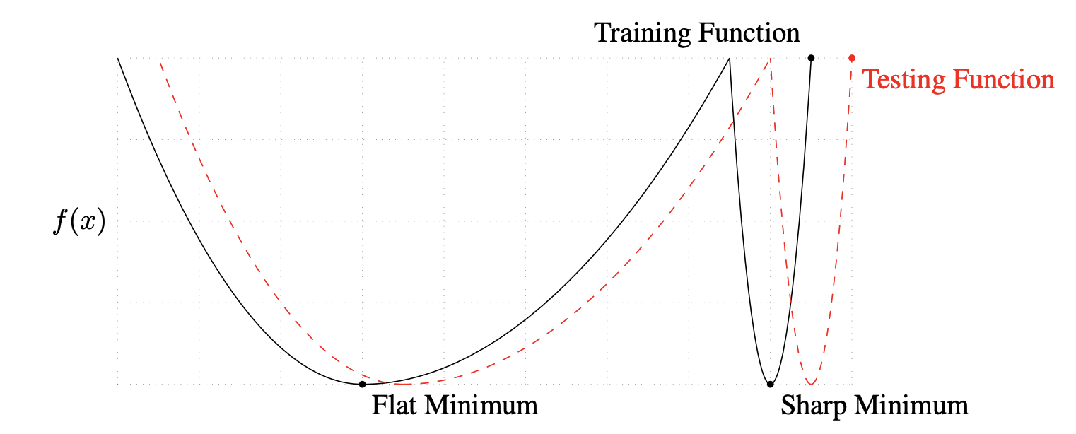
On Large-Batch Training for Deep Learning: Generalization Gap and Sharp Minima (Keskar et al., 2016). Data parallelism effectively provides a linear relationship between the number of available GPUs and the allowable batch size during training. This work empirically show that as we increase the batch size $B$, their models (applied to MNIST and CIFAR-10, both old and relatively small by today’s standards) begin converging to non-general solutions, which they attribute to large-batch solutions converging to sharp minima (e.g. areas of the loss landscape where the eigenvalues of $nabla^2 f$ are large), and not to overfitting (see Figure 25 above)Computing the eigenvalues of the Hessian is hard, so actually in the original paper they approximate the sharpness measure, which you can read about in the original paper.. So even if your model can fit on a single GPU, the effectiveness of data parallelism saturates as we scale. It has therefore become more interesting to cleverly parallelize our model computations across multiple devices.

III.2.b: Model parallelism

Like data parallelism, model parallelism is not necessarily that technically novel or interesting, but it is still extremely important and relevant today. Data parallelism relies on the model (+ optimizer states and data) fitting on a single GPU, but for large models this may not be possible (e.g. 400B parameter full-precision model is ~800GB just for model weights, far too big to fit on any GPU). AlexNet, for example, split the model across two GPUs in the original implementation, as they only had 3GB of RAM. Model parallelism is far more complex than data parallelism in that there are “blocking” steps — if we have a model with layer A which goes into layer B and we put the layers on different devices, we have to wait for layer A to finish before starting computation in layer B.

Mesh-Tensorflow (Shazeer et al., 2018). The core idea behind data parallelism is to split tensor computations along the batch dimension, which is free because model operations over these dimensions are entirely independent. In Mesh-Tensorflow, they propose an automatic strategy for splitting tensors along arbitrary dimensions (hence generalizing data & model parallelism) and scheduling them across multiple devices. The idea is that we can define a meshgrid of processors to handle tensor transformations in parallel, so this method does not reduce waiting times due to causal sequences of operations.

Another similar term you will probably see a lot is “tensor parallelism”, and it’s basically a form of model parallelism where we partition the weights of a layer along a particular dimension and place them on different devices. Megatron-LM, which we talk about in III.2.d, relies heavily on tensor parallelism.

III.2.c: Pipeline parallelism

Model parallelism & Mesh TensorFlow suffer from significant downtime when dependencies are involved. For example, if we split a model into layer A and B, where the output of A is the input of B, the devices holding layer B are blocked until layer A is finished. Pipeline parallelism is basically like pipelining in computer architecture — we pass partially computed tensors to satisfy dependencies, while also keeping GPU utilization high.

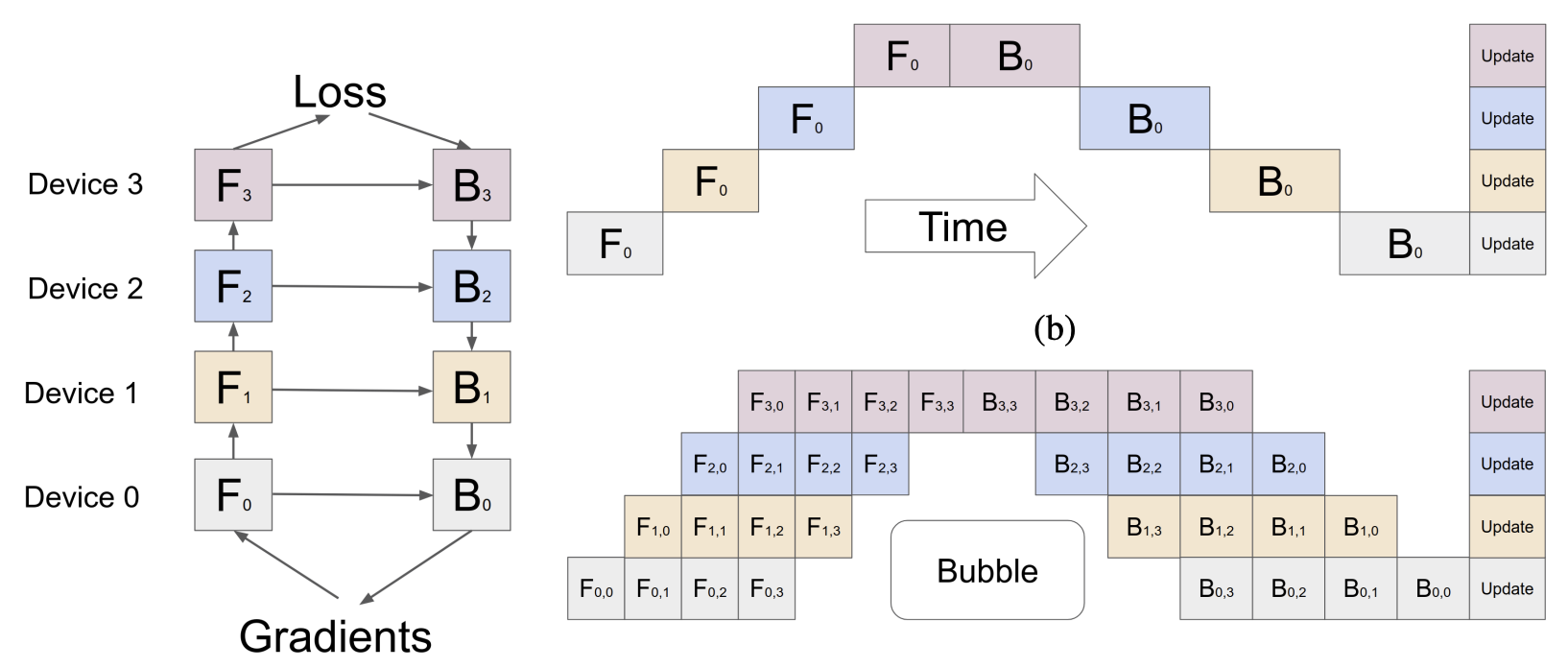
G-Pipe (Huang et al., 2018). One of the first open-source pipeline parallelism works for deep learning, G-Pipe is extremely simple and intuitive. To avoid stalls, they simply schedule sequential “micro-batches” on each device, so if device B has to wait for device A, it can process an earlier micro-batch while waiting for device A to finish its micro-batch. Like pipelining, there are bubbles that occur in this simple process, but compared to model parallelism, it significantly increases GPU utilization. They naively handle the backwards pass by waiting for all forward pass micro-batches to finish, due to the reverse layer-order dependency of the backwards pass. Finally, they perform a synchronous model update across all devices.

PipeDream (Narayanan et al., 2018). PipeDream was a concurrent work that developed a slightly different strategy. In addition to adding pipeline stages, they also interleave available backwards computations (e.g. when the first microbatch finishes its forward pass) with scheduled forwards passes to reduce bubbling caused by the reverse layer-order dependencies of backpropagation. PipeDream also features an automatic work partitioner for roughly dividing each pipeline stage to be equal in computation time. I didn’t talk about this in the context of GPipe, but uneven pipeline stages causes bottlenecks and therefore extra stall time.

Some other follow-up works like PipeDream-2BW (Narayanan, 2020) and WPipe (Yang et al., 2022) essentially minimize the stall / bubble time of the above methods, but are far more specific and still use the core idea that G-Pipe and Pipedream proposed.

III.2.d: Architecture-specific Parallelism

This mini-section is somewhat overlapping with the previous two, as model and pipeline parallelism are not necessarily architecture-agnostic. It should be pretty clear that there are certain considerations like load balancing and how to partition the model that are difficult to optimize when the model architecture is unknown. There are many recent works that focus on parallelizing specific architectures for scale, especially transformers.

Megatron-LM (Shoeybi et al., 2020). The aforementioned distributed training frameworks have pretty complicated implementations, and have evolved over time to include extra optimizations as well. The core thesis of Megatron-LM is to reduce overhead communication costs and assign operators in a Transformer models purely by intuition, and they identify synchronization points (basically where the devices will stall) that they can remove. Since then, Megatron-LM has changed significantly to be a framework for scaling languages, with two subsequent works https://arxiv.org/abs/2104.04473 and https://arxiv.org/abs/2205.05198, as well as a library called Megatron-Core for handling large-scale training.

III.2.e: Multi-node distributed training

We can generally get away with multi-GPU workloads on a single node (e.g. a DGX A100 8x80GB server) without having to deal with a scheduling algorithm or factoring node-to-node network bandwidth as a bottleneck, but as we start scaling even further to pre-training foundation models, we have to consider multi-node multi-GPU training frameworks.

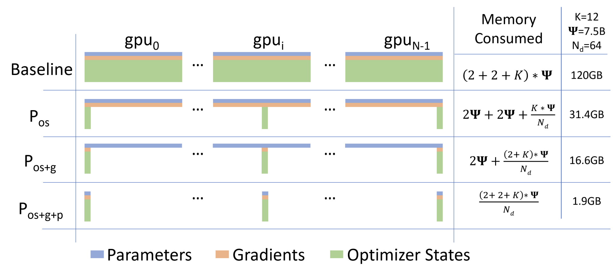
ZeRO (Rajbhandari et al., 2020). ZeRO cleans up most of the redundant memory footprint in data-parallel training schemes by partitioning across multiple devices / nodes. ZeRO is a family of optimizations separated into two classes: ZeRO-DP for “states”, and ZeRO-R for “residual memory”The paper introduces residual memory as activations, temporary buffers, and fragmented memory, but this is basically like the constantly changing / temporary data..

• ZeRO-DP targets various types of memory such as optimizer states (stage 1), gradients (stage 2), and the actual parameters of the model (stage 3). The general strategy is for each device to be responsible for holding and updating a partition of these components in memory, while requesting certain partitions only when needed (updates are made with a final all-gather or reduce-scatter). For example, when partitioning the model parameters, instead of performing model parallelism, where layer A sits on device 1 and sends its outputs to layer B on device 2, device 1 will instead grab layer B from device 2 and compute it all on device.
• ZeRO-R also centers around the partitioning strategy, but instead patches up a lot of the potential redundancies caused by ZeRO-DP. ZeRO-R handles activation checkpointing with a partitioning strategy similar to those found in ZeRO-DP (basically request it when you need it), but also uses a buffer to ensure requests are sufficiently sized while also handling memory fragmentation by pre-allocating contiguous memory chunks as needed.

There are a lot of rich details regarding how each optimization is ZeRO is implemented using node communication primitives that can be found in the original paper. ZeRO has since evolved into a family of optimizations for multi-device deep learning workloads and is directly usable with multi-device deep learning libraries like deepspeed.

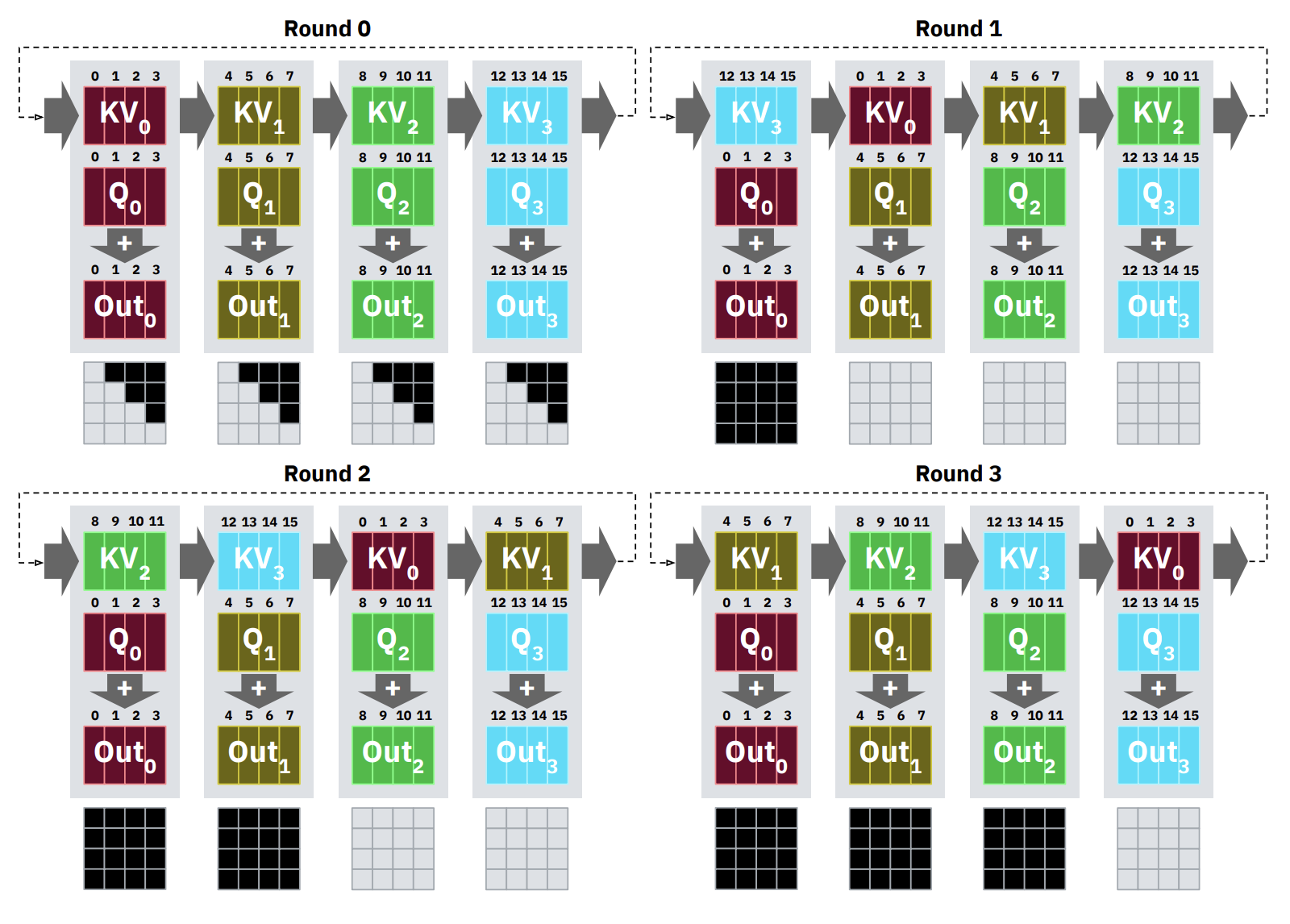
RingAttention (Liu et al., 2023) [unofficial code]. When we increase the effective context window of a model, we start getting to the regime where a single attention operation has to be split across multiple devices. Recall from our discussion of FlashAttention that we can compute attention by splitting $Q$ and $K,V$ into blocks. The Blockwise Parallel Transformer (BPT) takes this further by also fusing the subsequent feedforward layer with the attention layer, which operates independently on each $Q$ blockAllow me to clarify. When you look at FlashAttention, you’ll notice that the output block $O$ is computed by taking a block $Q$ with all the keys and values. In other words, $Q$ and $O$ are synced, and $K$ and $V$ are synced. Each FFN layer gets applied independently along the sequence dimension of the $O$ block, so we can apply it immediately when any $O$ block is computed.. RingAttention uses the intuition from BPT with one more observation: for every output block $O$, we compute it using a query block $Q$ and all key/value blocks, and the order that we load $K/V$ blocks is entirely permutation invariant! Thus, we can form a “ring” of host devices that each handle one query block, while we move each $K/V$ block from host to host to compute the $O$ block so each query block will see each $K/V$ block exactly once in some arbitrary order. This scheme overlaps the communication cost of moving around the $K/V$ blocks with the BPT computation, effectively hiding most of the latency that a naive distributed Transformer would have.

StripedAttention (Brandon et al., 2023)
StripedAttention is an extension of RingAttention that avoids redundancies caused by causal attention masks — instead of placing contiguous $K/V$ blocks on each device, they shuffle the keys/values to avoid completely masked out blocks (see Figure 28).

III.2.f: Libraries for distributed deep learning workloads.

Multi-GPU and multi-node algorithms like ZeRO have been integrated into libraries for developers to use. The community has moved extraordinarily fast on producing libraries for multi-device training and inference, making it possible for people with no knowledge to use multiple devices. In this section, I want to talk a little bit about those libraries, as well as provide some context for what is going on under the hood. We begin with a simple example of how to run basic distributed training in PyTorch.

PyTorch example. In PyTorch, we start by initializing a process group on each device that defines a master address/port, its device rank, the world size, and a communication backend.

• The master address and port from the master node, which generally controls the whole distributed system, is set across all nodes.
• The device rank or world rank is a unique identifier in $mathbb{N}$ for each device in the distributed network. The local rank is the identifier of a process within a node (e.g. gpu:0), and the world size is the total number of devices.
• The communication backend is the protocol that defines how messages are sent and received across nodes and devices, as well as the available communication collectives (e.g. send, recv, all_reduce, all_to_all, reduce_scatter, etc.).

# Define node-specific constants
os.environ[‘MASTER_ADDR’]= ‘127.0.0.1’
os.environ[‘MASTER_PORT’]= ‘01134’
torch.distributed.init_process_group(backend, rank=rank, world_size=size)

Modern libraries like deepspeed will make these primitives a lot easier for you, and will even make launching these applications with their CLI tools a lot simpler (you’ll probably just have to run deepspeed program.py ...). If you were to manually run a distributed workload (e.g. with PyTorch’s DistributedDataParallel or by defining your own sends and receives), you would typically have to run the program on each separate node while specifying their individual ranks.

Node communication backends. Under the hood, multi-node and multi-GPU workloads need to communicate and send data. Most libraries take care of this for you, but they will often have you define a communication backend — each of these serves a slightly different purpose and have various tradeoffs.

• nccl. NCCL is NVIDIA’s communication protocol specifically designed for inter-(NVIDIA)GPU communication. It is the recommended backend for most deep learning applications on NVIDIA devices.
• gloo. Gloo is more flexible for supporting CPU-GPU communication as well as GPU-GPU communication, and is often noted to be more useful for CPU-intensive distributed workloads.
• mpi. MPI has been the standard backend for most high-performance computing (HPC) applications.

Some relevant modern libraries. You can definitely code up a multi-GPU or multi-node job in PyTorch or TensorFlow, and most experienced developers choose to do this in favor of flexibility. However, there are many choices for libraries / CLI tools that handle multi-device training for you, and we list some in A.2: Large training / finetuning frameworks.

Part III.3: Scaling Laws

Characterizing model performance as a function of scale is a useful signal for whether any advances in efficient deep learning are even important. There are even works that look into predicting training curves, but in this section we mainly focus on observed empirical scaling laws and what they imply. All of the following scaling laws focus on characterizing the generalization / test loss in (nats/token), which is just the average negative log-likelihood with respect to the evaluation set. To keep this post focused on efficiency, I will mainly be glossing over results and leaving it to the reader to learn more about specific constant ranges or empirical findings.

Deep learning Scaling is Predictable, Empirically (Hestness et al., 2017). One of the first papers to present empirical scaling laws on a wide range of tasks (image, language, machine translation, speech) as a function of the training set size. They model test loss as a function of dataset size:

$$
mathcal{L}(D) = C cdot D^{alpha} + gamma
$$

and find that existing theoretical works estimate these constants incorrectly — prior works estimate $alpha sim -0.5$, while the empirical ranges they found were in $[-0.35, -0.07]$. Interestingly, they find in their experiments that the power law exponent $alpha$ changes across tasks, while $C$ changes based on model architecture and choice of optimizers.

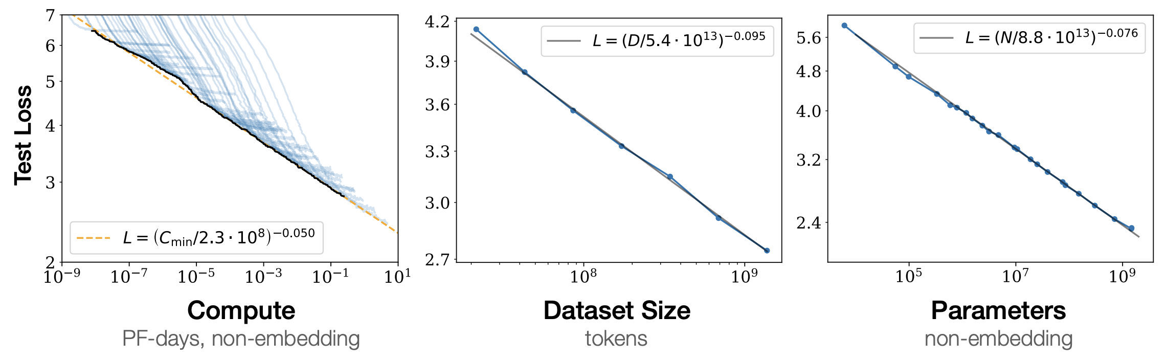
Scaling Laws for Neural Language Models (Kaplan et al., 2020). This paper proposes scaling laws across dataset size $D$, model size $N in [768, 10^9]$, and compute budget $C in [10^{12}, 10^{21}]$ FLOPS. They focus mainly on Transformer decoders on trained on WebText2, and they first analyze single-variable scaling laws by fixing $2/3$ of the above variables at a “sufficient level” and analyzing the third. They estimate in these models that each parameter costs roughly 6 FLOPS per token in the forward + backwards pass. These scaling laws are a power-law function of the test loss:

$$
mathcal{L}(X) = left(frac{X_0}{X}right)^{alpha} + gamma, quad X in {D,N,C}
$$

They notably discover through experimentation that:

• Counting embedding parameters for $N$ does not result in the nice power-law relationship we would expect, but excluding them does.
• Performance depends strongly on model scale and weakly on model shape, which is consistent with the findings of (Hestness et al., 2017).
• Increasing $N$ and $D$ at a fixed rate $N^{beta} / D$ is necessary to observe performance gains in the scaling laws.

They also derive test loss as a function of multiple variables, which are consistent analytically when you take the limit of one variable (think of it as a form of marginalization). Using this function, they propose an optimal allocation of resources given a fixed compute budget. For specific coefficients and rationale for their fitting functions, I would highly recommend reading the original paper — they have a lot more conclusions and experiments than what I’ve discussed above!

Chinchilla (Hoffmann et al., 2022). This landmark paper in neural scaling laws for LLMs is a collection of over 400 large-scale experiments (all Transformers with a cosine schedule learning rate and trained on one epoch), entering the foundation model range (70M – 16B parameters, 5B – 500B tokens) that (Kaplan et al., 2020) does not touch on. From an efficiency perspective, they are interested in optimal cost budgets, i.e.

$$
N^*, D^* = underset{text{FLOPS}(N,D)leq C}{text{argmin}} mathcal{L}(N,D)
$$

In their experiments, they vary both the number of training examples for a fixed model size and the model size for a fixed FLOP budget, and fit (+ motivate) the scaling law according to the function (with fitting parameters $A_0, A_1, alpha, beta, gamma$).

$$
mathcal{L}(N, D) = frac{A_0}{N^{alpha}} + frac{A_1}{D^{beta}} + gamma
$$

Under their fitted power law, they set a constraint budget $6ND leq C$ for their proposed compute-optimal Chinchilla model. In the domain of large language models, scaling law papers are hard to come by because of the sheer cost of running experiments. Other works like Beyond neural scaling laws, Transcending Scaling Laws with 0.1% Extra Compute, and Scaling Data-Constrained Language Models explore how scaling law constants change under different datasets, constraints, and model assumptions. From an efficiency standpoint, there will always be interest in deriving the upper-bound of power law constants $alpha,beta$.

Part III.4: Revisiting downwards scaling

A natural analogue for neural scaling laws is the lower bound of compute necessary to achieve some level of model performance. In the era of foundation models and Transformers, model compression methods have evolved to deal with the challenges of large-scale models trained on huge datasets.

III.4.a: Small Language Models (SLMs)

With foundation models getting too large to fit on affordable hardware, there has been a growing interest in how to train a small language model that performs the same as a large language model. A lot of the subsequent sections are relevant to training SLMs from scratch and from an LLM.

The Phi models. The Phi models are a series of open-source SLMs from Microsoft Research designed to emphasize the value of high-quality training data. This idea may contradict the scaling laws we discussed in the previous section, but actually the scaling laws bake in assumptions such as properties of the data distribution, types of models used, etc. that aren’t universally covered.

• Phi-1 (Gunasekar et al., 2023). phi-1 is a 1.3B parameter model trained on 6B tokens of high-quality scientific/textbook material for coding. Compared to other models at the time, which were generally 10x bigger and trained on 100x more tokens, it displayed near-SOTA performance on HumanEval (Pass@1) and MBPP (Pass@1), which were the primary coding benchmarks at the time.
• Phi-1.5 (Li et al., 2023). As a follow up, they build more 1.3B parameter models trained on “textbook-quality” data generated by LLMs and show near-SOTA performance on reasoning tasks beyond coding! It’s unclear how the learned distribution is affected by this synthetic training data trick, but for Phi-1.5 it seems to work fairly well.
• Phi-2, Phi 3, Phi-3.5 (Microsoft, 2024). Subsequent iterations of the Phi models were larger (~2-3B parameters) and trained on significantly more high-quality filtered & synthetic “textbook” data. They demonstrate the capabilities of these models across language, vision, and multi-modal tasks, and also introduce a mixture-of-experts version (~6B params) to compete against models of a similar size like LLaMA 3.1, Mixtral, GPT-4o-mini, and Gemini-1.5-Flash.

Similarly sized models follow the same training recipe (i.e. really “high quality” data seems to affect the power law constants positively), but not all of them are open-source.

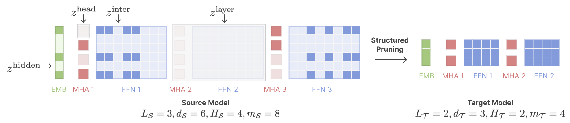
Sheared LLaMA (Xia et al., 2023). Existing pruning techniques mentioned in II.6.a: Model Pruning have found little success in the large language model space due to the lack of hardware-aware structure. Instead, in this work they prune at a higher abstraction such as the number of layers, attention heads, and hidden dimensions to enable hardware-aware structured pruning for language models. They also introduce “dynamic batch loading”, which is an online optimization-style problem for adjusting the proportion of data from each domain that is added to the training batch. I am hopeful that more theoretically motivated versions of this technique will be useful for faster convergence.

Knowledge Distillation (KD).I apologize for keeping this section brief. I think KD is a very rich field, but there just isn’t much to talk about except how to improve matching the distribution of one model to another. In terms of “efficiency”, I don’t have that much to say about the topic. Knowledge distillation emerged around the time when other methods like pruning and quantization were popularized, but the more interesting ideas like black-box knowledge distillation came about due to the closed nature of a lot of large models. Generally, the idea is to start with a large language model (teacher) and produce a small language model (student) by “distilling” the behavior of the large language model into the small language model.

• White-box KD means we have access to the logits/distribution of the large teacher model, and our optimization objective is to align the distribution of the student to the distribution of the teacher (e.g. through KL divergence). MiniLM claims that KL is not the right optimization objective for language, but works like Baby LLaMA have shown that standard white-box KD can yield good results.
• Black-box KD is interesting in the era of large models because many SOTA LLMs are available through APIs. One of the more interesting techniques is Zephyr, where they fine-tune a small open-source model with SFT + DPO by generating (instruction, response) pairs from a larger closed-source model. Given the fact that people train their models on synthetic model-generated content (e.g. GPT-4), it is not that surprising that black-box KD works in this wayAs a side note, I wonder what this implies about the distribution of “language” we are learning and what kind of space it lies on..

III.4.b: Modern quantization techniques

We revisit the topic of quantization and some popular research directions related to it. Quantization is especially interesting for language models because it can be made efficient for modern hardware without affecting the architecture of the model. However, unless the entire model is quantized, quantization methods still suffer from a lack of hardware support for speed-ups.

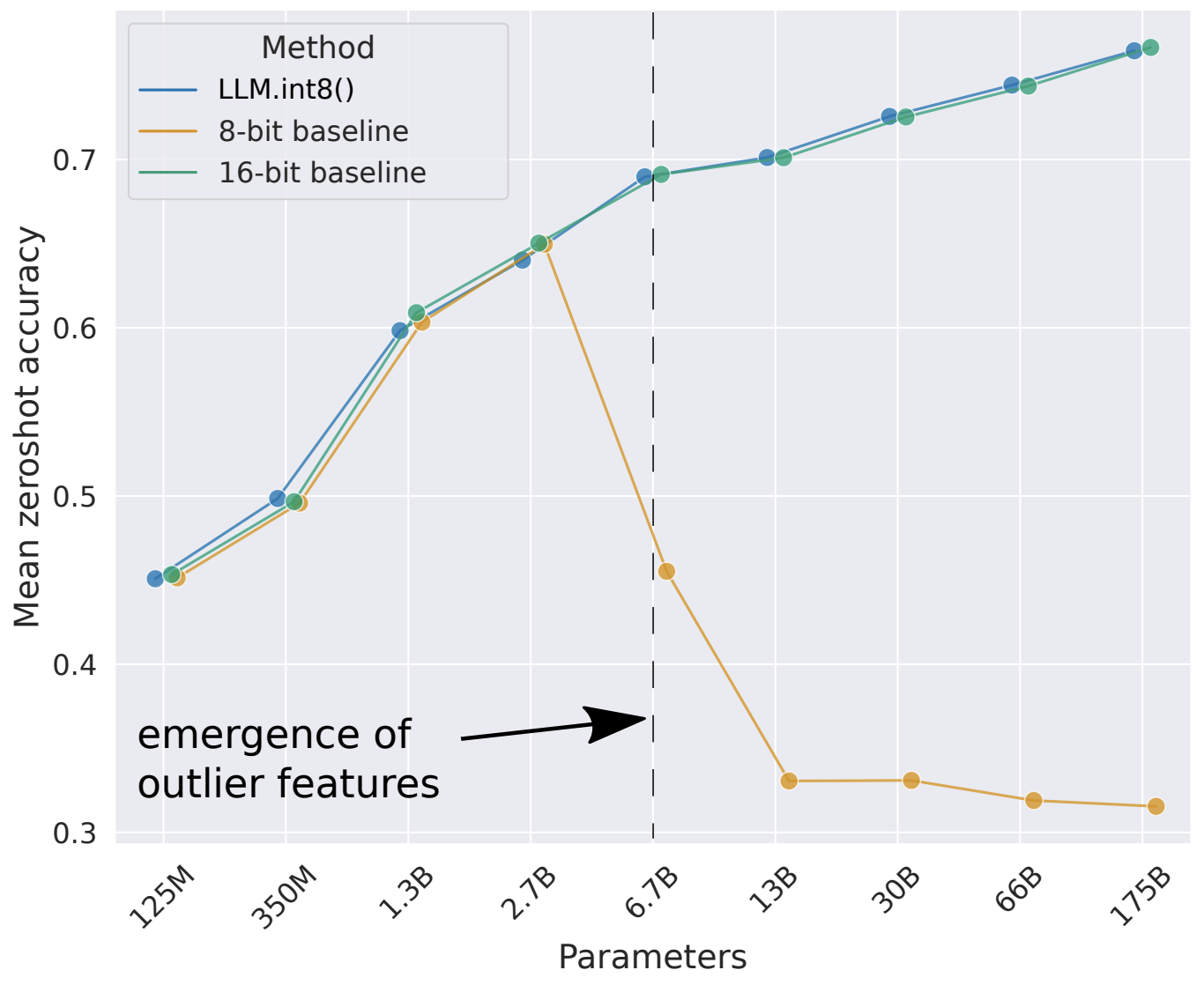
LLM.int8() (Dettmers et al., 2022). While FP32 and FP16 (+ mixed precision training) have been shown to work fairly well with LLMs, this work was the first to perform 8-bit (INT) quantization for large-scale LLMs. The authors discover that <1% of input features have a high variance/magnitude, which causes a large quantization error when going down to 8-bit representations. They also find that this “outlier” phenomenon occurs along the same hidden dimensions across most sequences, so they separate these outliers out using an outer-product notation for matrix multiplication. More formally, for outlier dimensions $O$,

$$
XW = sum_{o in O} X_{:,o}^{fp16}W^{fp16}_{o,:} + sum_{k notin O} X_{:,k}^{int8}W^{int8}_{k,:}
$$

Lastly, they assign quantization constants to each row of the input and each column of the weight matrix (vector-wise quantization). Interestingly, they attribute model collapse in Figure 31 to quantization errors propagating across all layers in larger models.The author of LLM.int8() and QLoRA (Tim Dettmers) has also built the [bitsandbytes](https://github.com/bitsandbytes-foundation/bitsandbytes) library for quantizing / fine-tuning LLMs using these techniques. It is an extremely simple and popular wrapper around Huggingface transformers for quantizing your models!

GPT-Q (Frantar et al., 2022). Following the same trend as before, GPT-Q quantizes LLMs to the 4-bit regime while stably reducing generalization perplexity for large models. They focus on layer-wise quantization, meaning they isolate each layer and do not consider layer-to-layer effects. Following the Optimal Brain quantization framework, they minimize the following quantization error:

$$
text{argmin}_{W^q} | WX – W^q X |_2^2
$$

Intuitively, what we’re doing here is quantizing a row of the weights, then adjusting the full precision weights to minimize the error, and iteratively performing this update. There are closed form solutions to this iterative update by Taylor expanding the error above that were originally derived in (Optimal Brain Surgeon, 1992), but GPT-Q modifies/approximates the algorithm to maximize GPU utilization. Like other quantization methods at the time, quantizing the rows at different granularity did not enable any speed-ups on GPUs.

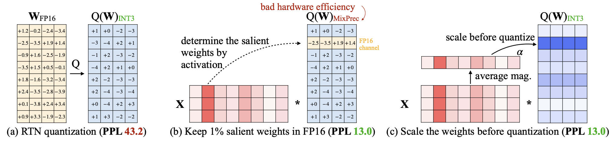
Activation-Aware Weight Quantization (AWQ) (Lin et al., 2023). The authors observe in experiments that only a small percentage of weights in an LLM are “salient”, meaning they are extremely sensitive to quantization. Furthermore, they observe that the saliency metric is dependent on the input data (i.e. the activation resulting from the weight times the input). Thus, prior to the post-quantization step, they sample a subset of the original data distribution and find the high-variance activations to determine salient weights (see Figure 32.b). Instead of keeping these salient weights at full precisionFrom a hardware perspective it’s always hard to intermix weights at different precisions because 1) you need kernels that can handle this and 2) the way it’s stored in memory is not convenient — imagine implementing a C-array that can take multiple types. Indexing into the array with pointers would be a pain., they find in theory that adding a computed scaling factor can reduce quantization error without affecting the range of representable values (see Figure 32.c). They demonstrate their method by using 4-bit AWQ on LLaMA-2 70B to deploy on a single NVIDIA Jetson Orin 64GB.

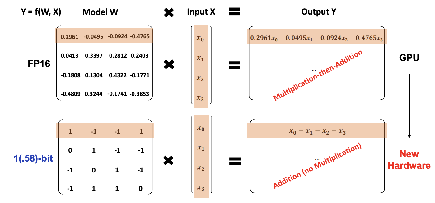
BitNet (Wang et al., 2023). Another research direction that emerged was quantization-aware training, where a model stores weights and gradient updates in full precision, but computes the forward pass in the quantized regime (a straight-through estimator is used for gradient computation). BitNet replace all linear layers (e.g. nn.Linear or just the $W$ matrices) with rounded 1-bit variants (i.e. $W_{i,j} in $ { $-1,1$ }) and quantize the activations to 8-bits with absmax quantization. While BitNet was a cool experiment, the results were subpar compared to other existing quantization techniques, and the produced model was not any faster on existing hardware than a standard LLM.

BitNet b1.58 (Ma et al., 2024). A follow-up and arguably more successful variant of BitNet was the ternary version (i.e. $W_{i,j} in$ { $-1,0,1$ }). The recipe is basically the same, except they compare to a half-precision LLaMA {1.3B, 3B, 7B, 13B, 70B}, and demonstrate better / comparable performance on a wide range of language reasoning tasks, as well as significantly faster throughput (up to 10x) and less active memory usage (up to 4x reduction)I have very little intuition as to why this paper does so much better than BitNet (maybe something key about LLaMA models?) and I think this paper should do a better job of explaining it as well. As much as I want to believe something like this works, it seems almost too good to be true in most practical settings. I hope some more follow ups investigate the “whys” that this paper leaves open.!

SmoothQuant (Xiao et al., 2023). Most of the aforementioned methods focused more on memory reductions rather than speed improvements. Like other papers, the authors observe that outliers cause a lot of problems for quantization schemes. SmoothQuant chooses to work entirely in the quantized regime for both weights and activations without needing to dequantize anything. Because we can’t control outliers in the activations (this is input dependent) but we can control the initial distribution of weights, SmoothQuant adds a per-channel scaling factor based on a calibration setSimilar to what AWQ does (from the same lab), they use calibration sets as an approximation of the data distribution. to scale down outlier activation channels, and a corresponding inverse per-channel scaling factor to the weight matrix. Effectively, they squash outliers in the inputs by introducing some outliers to the weights, which they argue is better than large outliers.

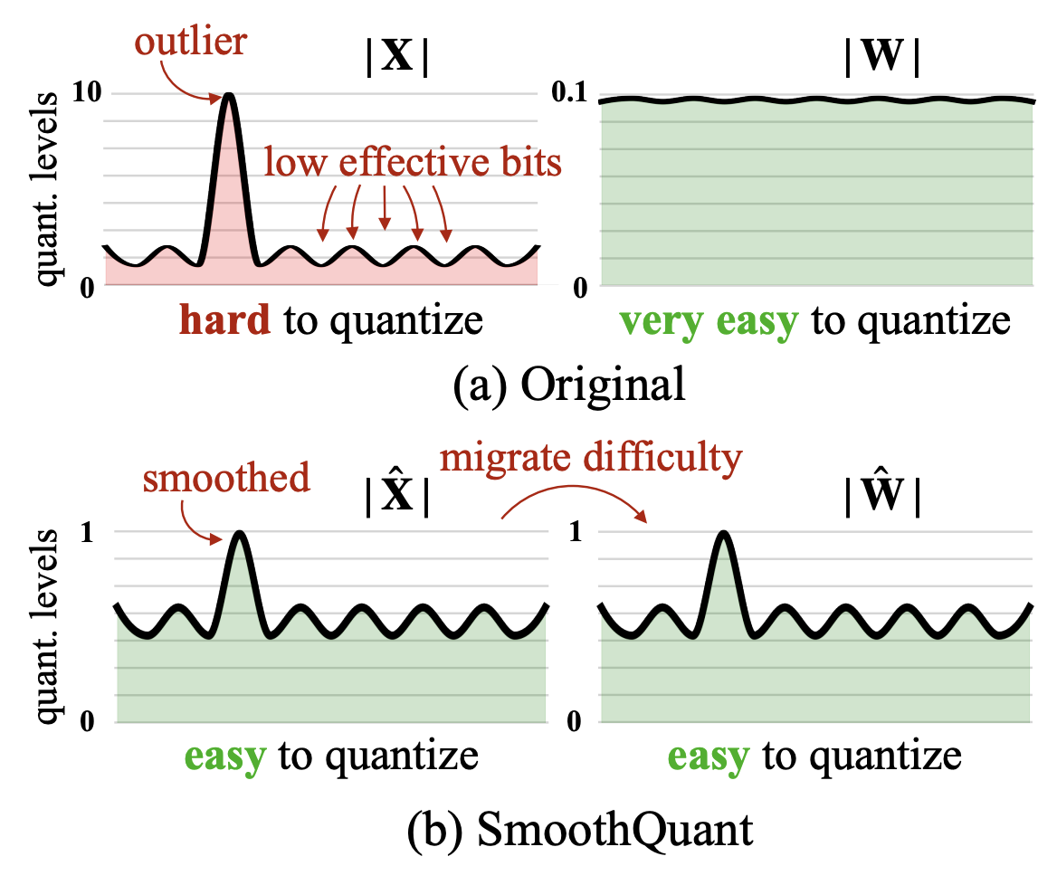
Under this scheme, we never need to go back and forth between different precisions, so we can directly apply low-precision kernels that enable speed-ups!

III.4.c: Sparse Parameters

One research direction that hasn’t really taken off for the past few years is introducing sparsity or sparse decompositions to model parameters. We mentioned in III.1.a: Shaving complexity: Approximate Methods that sparse attention methods were just not efficient on modern parallel processors, which is not entirely true(-ish).

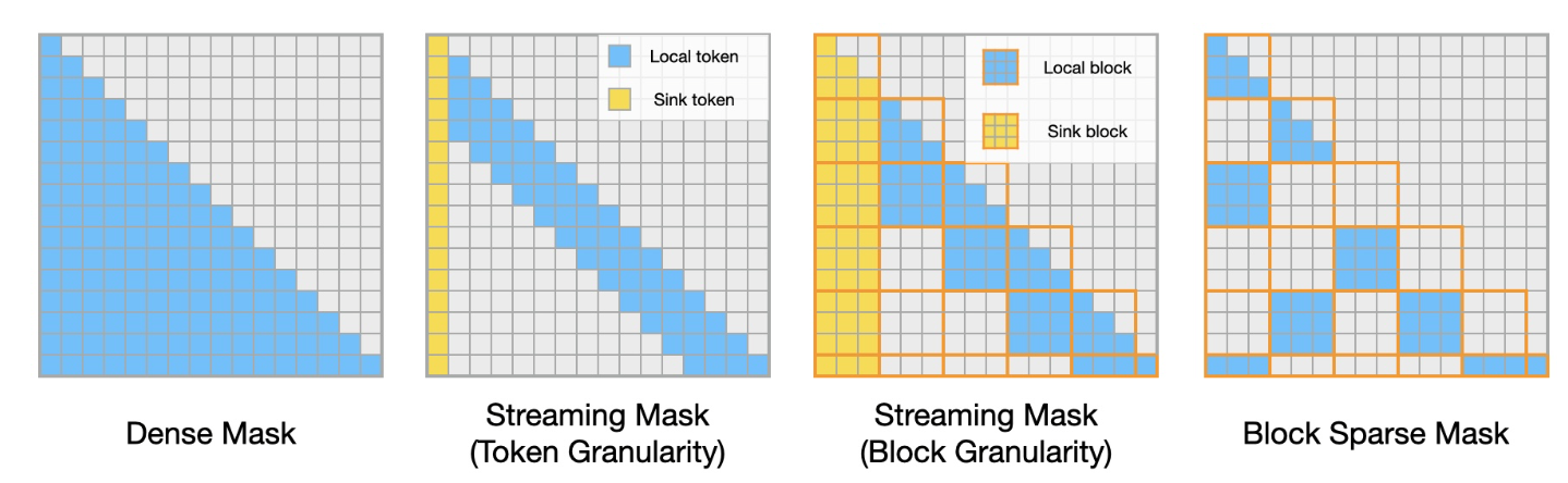
StreamingLLMs with Attention Sinks (Xiao et al., 2023). It should be somewhat clear by now that pre-defined sparsity patterns can be made efficient on GPUs. In this work, they return to window attention masks (causal mask that can only attend back a certain length) and add the ability to attend to a fix (set of) “attention sink” tokens, which they hypothesize contain global information due to the inherent structure of the attention mechanism. Furthermore, the authors develop efficient fused kernels in https://hanlab.mit.edu/blog/block-sparse-attention for efficiently handling these sparse patterns.

Sparse factorizations. One really interesting direction a few years back was factorizing model layers into sparse parameters, but ultimately it didn’t really take off. I am hopeful that people continue working on this direction, because derivable factorizations can say something about how our models work.

• Butterfly Matrices (Dao et al., 2019). In this work, they show that a large class of structured matrices (e.g. FFT, DFT live in this family) can be recursively factorized into sparse matrices with a nice block diagonal structure. While the implementations are not hardware friendly, these factorizations theoretically lead to a reduced number of operations and memory-footprint. I really
• Monarch Matrices (Dao et al., 2022). As a follow-up, they derive a less-expressive class of matrices with hardware-friendly factorizations. Despite now being practically interesting, I haven’t seen much follow up work in this area in recently.

Part III.5: What about model inference?

The introduction of ChatGPT (2022) made it clear that building infrastructure to support querying large models ( i.e. model serving) was a necessary research direction. In addition to the compiler optimizations offered by inference engines like TensorRT for speeding up model code, people also began thinking about how to handle and schedule batches of user requests. The primary considerations were minimizing the latency of each user request, and maximizing the throughput of processing all user requests. Furthermore, due to the nature of KV-caching that we discussed in III.1.0: Early Insights, these systems generally have to distinguish between the pre-filling stage, where an initial prompt is fed into the model and all keys/queries/values are computed, and the decoding phase, where cached KVs can be re-used, and only one new query token is considered.

llama.cpp (Gerganov, 2022). One of the coolest solo projects by Georgi Gerganov is a pure C++ implementation of the LLaMA family that optimizes for non-GPU devices (it now supports GPUs). It has since become a standard tool for running model inference on a variety of language models, and is extremely simple to use with its CLI. The downside is that adapting this code for custom LLMs is difficult without a strong understanding of the underlying implementation.

III.5.a: Generative model serving

The most naive form of model serving for generative Transformers is to batch a bunch of requests, process them, then distribute the results back to each user. There are a lot of annoying considerations like non-uniform length prompts, non-uniform length generations, and how to handle the KV cache in memory (which is not small!) that people quickly began figuring out in the past two years.

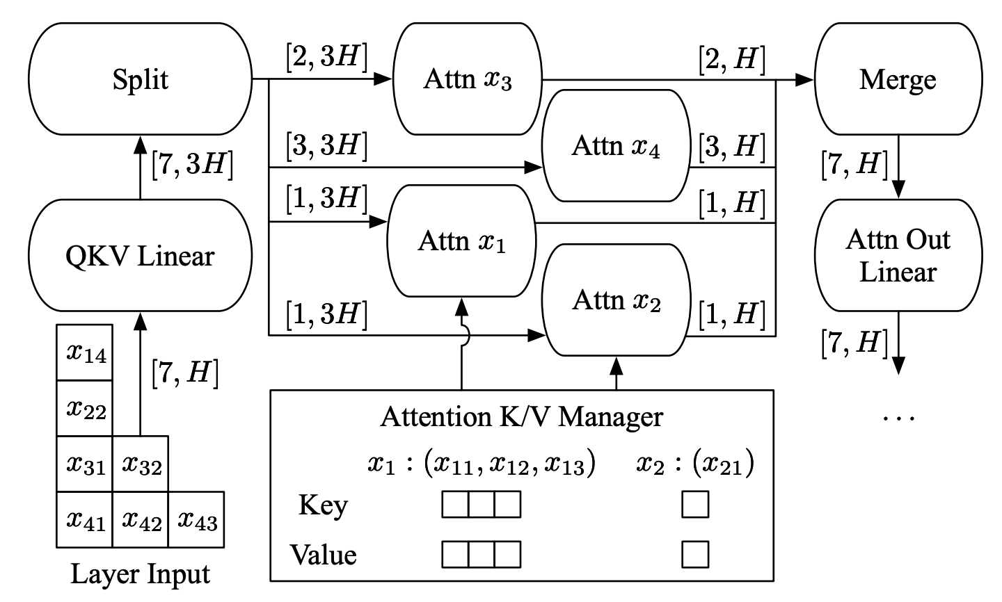
Orca (Yu et al., 2022). One of the first open-source engines for model serving optimized for throughput. Given a batch of requests, their scheduler works at the token-level (they call it iteration-level), meaning it doesn’t care if two requests were launched at different times. Furthermore, they notice that certain operations in a Transformer in non-batchable requests (e.g. they’re in different stages or of different lengths) can actually be batched — any linear transforms can be batched regardless of length (see Figure 35).

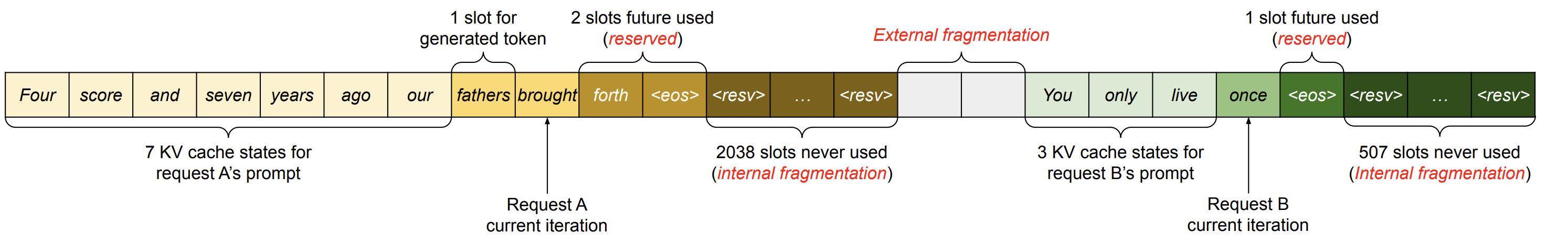
vLLM and PagedAttention (Kwon et al., 2023). Keeping the KV cache on the same device is critical for keeping model throughput high, as it avoids overhead communication costs. However, prior works like Orca handle the KV cache naively — they generally pre-allocate a fixed length memory buffer for the KV cache, which causes several memory inefficiencies highlighted in Figure 36. Furthermore, these methods have no way of sharing KV caches for shared prefixes across multiple requests. PagedAttention mitigates these issues by introducing ideas from virtual memory in an operating system — they block up the KV cache into equal and fixed size chunks and use a translation table to map them to physical DRAM. Equivalent chunks in different requests get mapped to the same physical memory, enabling memory sharing. While the KV blocks are not contiguous in physical memory, the elements in the block are locally contiguous and internal and external fragmentation are significantly reduced. vLLM is a serving engine on top of PagedAttention that operates at the request level (batches according to request arrival) and handles the virtual and physical KV cache for a variety of common decoding methods on single and distributed hardware.

Sarathi-serve (Agrawal et al., 2024). Prefilling (high latency, high GPU utilization) and decoding (low latency, low GPU utilization) are difficult to schedule together, but serving systems will often having many concurrent requests at either stage. The authors observe that when optimizing for throughput or greedily scheduling prefills first, there is a tradeoff between the time-between-token (TBT) chunking prefills to interleave requests at a finer granularity and 2) interleaving ongoing decodes with other requests to prevent stalling ongoing requests. tldr; if you optimize too much for throughput, you’re inevitably going to make some requests really slow. Sarathi-serve tries to make sure no request gets stalled for too long while still maximizing throughput.

III.5.b: Fast decoding strategies

We have mentioned over and over again that many Transformer computations are memory-bound, and this is especially true for model inference. While we can increase inference throughput using the methods in the previous section, the latency is lower-bounded. A new research direction on fast decoding strategies has emerged to push this lower bound down.

Speculative decoding (Leviathan et al., 2022). The core idea is to sample tokens from a cheaper “draft” model $q(x_{<t})$, and use a cute probability trick to make sure the distribution we sample from is actually the large model $p(x_{<t})$Up until now I’ve tried to avoid writing out math because I always recommend reading the original paper if you’re more curious about the “why”, and in this case the original paper is really simple, so I think it’s much easier to just let the math speak.. The savings comes from the fact that we can actually sample multiple sequential tokens from $q(x_{<t})$ while simultaneously computing tokens and the actual distribution from $p(x_{<t})$. We can then perform rejection sampling based on the likelihood of the generated token, and choose up to the first token that was rejected. By using more compute resources, we can speed up decoding by up to how much faster the smaller model is than the larger model. This work was critical for future ideas on using smaller models for faster decoding.

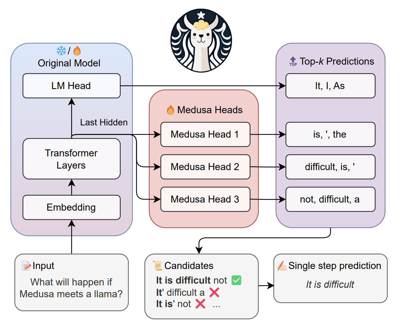
Medusa: Multiple Decoding Heads (Cai et al., 2024). Instead of using a smaller draft model, which is hard to fit into the GPU memory hierarchy without being slow, Medusa uses multiple prediction heads (each head is just a FFN with a residual connection) at the last hidden state and a sparsely structured attention mask over the predictions (basically to make sure they only attend heads can’t attend to tokens they didn’t generate) which they call “tree attention”. Unlike speculative decoding, the authors argue that matching the original model distribution is unnecessary, as long as the outputs are “reasonable” (they define a rule based on truncated sampling).

Part N: Modern Day and Beyond

We are still in the era of scale. However, in my opinion (not necessarily shared by the community), I don’t find the recent results of “scaling” to be particularly impressive (e.g. in a lot of the domains like decision-making game environments, software engineering tasks, etc. LLMs are still pretty bad). A lot of the prior directions in Part III are still being tackled to this day, so this section will feel a bit all over the place. Here, I will list some interesting on-going threads without a strong answer.

N.1: What’s up with these superclusters?

I recently listened to this Dwarkesh podcast with Leopold Aschenbrenner where they talk in the beginning about the huge cost of building compute clusters that can support scaling model training. They talk about the natural progression of scaling these data centers beyond to 100K H100s, ~150 MW, and then to 1 GW, and beyond. GPT-4, for reference, was rumored to be trained on ≥20k A100s with 13T tokens, or roughly 2e25 FLOPS. It’s also been rumored recently that Microsoft wants to build a 100 billion dollar data center/supercluster for their AI applications.

Obviously we haven’t observed the ceiling of the “scale to model performance” relationship, but I’ve always been a bit irked by the rush to continue scaling to uncharted territory, where the superclusters in AI are finally surpassing the existing institutional superclusters. I get that it has been “working” for a few years, but in some sense it reached a level of performance that I don’t find particularly surprising. LLMs model the distribution of language in its data distribution quite well, and they “generalize” to novel tasks (what does generalization even mean? We can barely characterize the distribution we are feeding as training data so what we think is generalization could be trivial when the model optimizes with respect to the entire Internet). Even more concerning, how did we extrapolate to the idea that these newer models will be superintelligentI’m not claiming AI cannot be dangerous. In fact, existing AI applications are already dangerous in not-so-sci-fi-esque ways. I also am not denying that safety / doomsday preventative research is important. But for “scale-pilled” individuals, the argument for burning billions of dollars seems a bit weak. I wonder if there is some strong prior about the equations or models we’ve been using that people have been seeing., or even that much more useful for that matter? Why is a GPT-7 that much more useful than a GPT-4?

Remark. I’m genuinely just curious what the rationale is, and I wonder if someone has a good answer for me. I would love to see a supercluster get built because I think it’s cool, but realistically there’s a high probability that it turns out to be a massive waste of resources.

N.2: How much bigger are industry resources than academia?

So I graduated from Princeton this past May, and during my undergrad I was part of the Princeton NLP group — now rebranded as Princeton Language and Intelligence (PLI). At the tail end of my time there, it was announced that PLI had purchased 300 H100 GPUs, positioning itself as one of the largest academic clusters for deep learning. The only other comparable academic cluster is UT Austin’s 600 H100 cluster, which most research labs would love to have.

I got curious about these numbers, because Meta’s LLaMA 3.1 family was reportedly trained on 16k GPUs on their 24k GPU cluster (I wonder what kind of monstrous network topology they’ve built…) — in this blog, they estimate training to take ~100 days on this cluster (not sure how accurate this estimate is but this ballpark seems somewhat reasonable given the FLOPs range). And this is just on Meta’s LLaMA team — I’m sure they have more compute spread out across the company. In other words, my academic lab doesn’t seem so grand in comparison. That’s not to say that you cannot do good research in academia, but it is pretty funny to me just how much more compute and money these industry labs have over some of the most prestigious academic labs in the world.

N.3: How fast can we train old models with modern techniques?

I’ve always been curious how fast we can train older algorithms on new hardware with all the new fancy tricks we’ve learned throughout the years. Here is a thread of some interesting works in this direction.

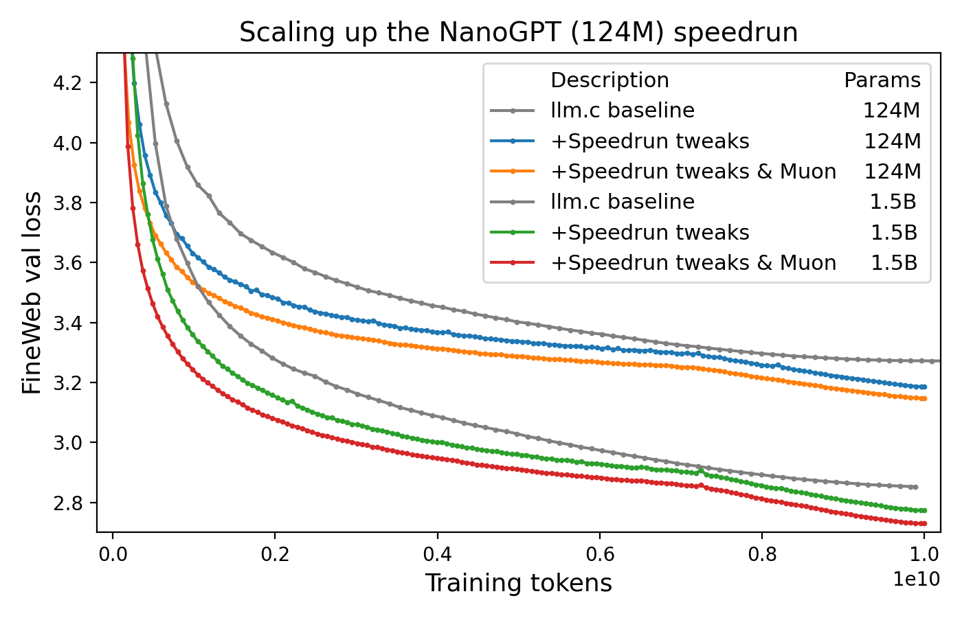
llm.c to speedrunning NanoGPT (Keller Jordan, 2024 – ).
Andrej Karpathy’s super efficient implementation of GPT-2 (124M parameters) called llm.c achieves a validation loss of 3.28 on FineWeb in 45 minutes on an 8xH100. This feat was further pushed by an ongoing Twitter thread on applying modern training techniques to tweak the NanoGPT model to converge faster.

• The original thread adding rotary embeddings and an increasing LR. 31.4 min.
• Using new muon optimizer, although I don’t fully understand the intuition or what exactly it does (some kind of fast orthogonalization trick applied to the Nesterov momentum update). It does use less memory than AdamW though and is slightly faster! 24.9 min.
• The rest of the changes are in the repo/on Twitter, but it’s of the flavor of 1) tuning muon, 2) tweaking activations and layers 3) hardware-aware tricks. Current record: 12.03 min.

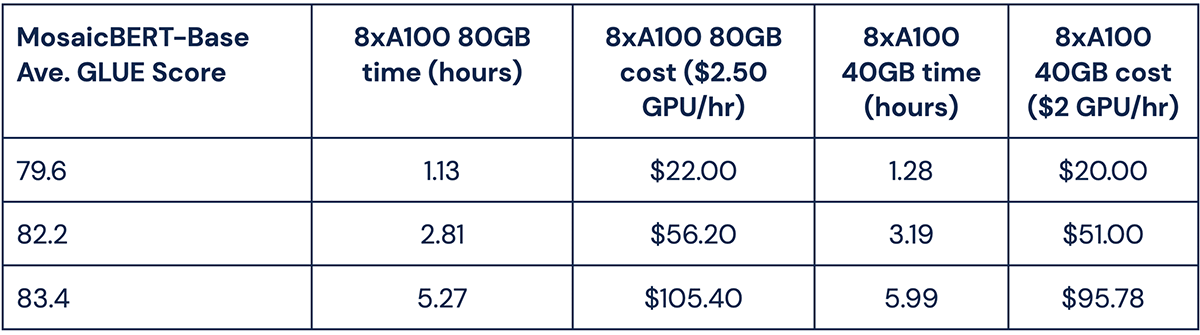
Pre-training BERT for under $20 (Mosaic AI, 2024). I really like this blog, as it showcases how far we’ve come in deep learning efficiency. BERT and RoBERTa were some of my first introductions to the field of deep learning, and they were known at the time to be some of the biggest training jobs, costing upwards of $300 and taking >4 days on 16 TPUs! They use a suite of tricks like FlashAttention, ALiBi, and unpadding, as well as the popular C4 corpus for pre-training. Basically, this paper takes the original BERT model and trains it entirely differently while using modern hardware and libraries, and it turns out to work extremely well. I’m excited to see how fast we can train LLaMA 3.1 405B in the future!

N.4: Recent efforts to scale hybrid or non-Transformer.

I sort of briefly mentioned alternatives to Transformers like SSMs and relevant algorithms like FlashFFTConv that are used to accelerate them. Given the existing constraints of Transformers and the attention mechanism, I wanted to discuss some alternatives and roughly why people have been interested in them.

• Transformer-SSM Hybrids (e.g. Jamba, Striped Hyena). These models attempt to combine SSM blocks with Transformer blocks to improve long context reasoning capabilities. These models are still in the early stages of research without a key production-level model, but I wouldn’t be surprised if something interesting emerged from them in the future.
• RWKW. An open-source effort (led by BlinkDL) to build an RNN that can be trained with parallel algorithms like a Transformer while maintaining constant memory / compute complexity during inference.
• RetNet (Sun et al., 2023). Reformulating the attention mechanism with a recurrent formulating to get the benefits of a Transformer-like architecture with constant compute complexity during inference. It aims for similar guarantees to RWKV but the approach is entirely different.
• Linearizing Transformers (e.g. Distilling Transformers into RNNs, Linearizing LLaMA 3). These methods attempt to take pre-trained Transformers and somehow distill or convert them into a different model with better inference-time guarantees. Unfortunately, the performance hit seems to be pretty significant in a lot of these.

N.5: Model efficiency Benchmarks

We have a lot of benchmarks for evaluating model performance, but not as many for evaluating efficiency. The most comprehensive benchmark available is the MLPerf benchmarks, which features inference, training, and HPC tasks across a wide range of modalities. In most instances, we can directly just compare algorithms on specific hardware, but I would be interested in more rigorous benchmarking in the future.

N.6: Startups in the Efficient Deep Learning Space

I have no affiliation to any of these startups — I just came across these at some point in the last year and felt they were interesting enough to save in my Notes app. I have no way of verifying if the work they’re doing is legit or even useful, so take it all with a grain of salt.

• Etched. An ASIC specialized for Transformers. At the time of writing, little information is known about their chip.
• Cerebras. Develop specialized chips for AI applications, with gimmicks like lots of on-device memory and super-fast inference for large models.
• Together.ai. They’re pretty well known for their open-source work and research on fast inference methods and Transformer-SSM hybrids, but they also have a cloud platform for fine-tuning and using a wide variety of large models.
• Groq. An ASIC specialized for language (basically big model) AI applications. They remove a lot of the complexity with CUDA’s hierarchy, and instead focus on being super low-latency and energy efficient. As far as I understand, they’ve mostly been used for model inference, like a lot of the other ASICs mentioned.
• Tenstorrent. They develop a lot of custom hardware from chips to workstations specifically for AI applications. From what I can tell, they’re trying to build out a whole CUDA-like ecosystem, but I’m guessing they’ll need some kind of breakthrough performance to attract more interest.

Resources

A.1: Where to access “free” GPUs?

There are plenty of services like Amazon AWS, Google GCP, Microsoft Azure, etc. that offer cloud GPUs, but if you’re not rich like me, you may also be interested in what free options are currently availableGradient by Paperspace used to be my go-to, but I can’t seem to find what happened to it..

• Google Colab. You can get access to a free Tesla T4 16GB when using their notebooks, but the time limits are not consistent and you’ll have to use multiple emails to get consistent usage.
• Amazon SageMaker Studio Lab. Another notebook service with a Tesla T4 16GB available with just an email! The time limits are also not great on this one.
• Lightning.ai. You get 22 free GPU hours every month without needing to put in a credit card, and you also get a vscode-like interface so you can just plop in your codebase and run what you need.
• Kaggle. Kaggle gives access to free NVIDIA K80s with a weekly limit. I’m not sure what it is anymore, but it used to be 30 hours/week.

A.2: Large training and finetuning frameworks.

There are many options for handling large-scale training jobs other than PyTorch/TensorFlow’s in-house wrappers and distributed modules. A lot of these examples use config files or YAML file configurations for defining your desired job. We list some useful libraries below.

• torchtune. Torchtune is PyTorch’s newest module for fine-tuning large language models. They’ve heavily modularized their code and have some nice recent examples with LLaMA 3.
• HuggingFace PEFT. PEFT integrates most of the existing parameter-efficient fine tuning (recall from III.1.c) methods to work with models loaded from the Huggingface transformers library.
• accelerate. A super-thin wrapper around your PyTorch models, dataloader, and optimizer for launching multi-GPU jobs without a lot of extra code.
• deepspeed. A library around PyTorch for reducing multi-GPU workloads automatically. It notably integrates ZeRO optimizations, and works really well with / similarly to accelerate.
• axolotl. A fine-tuning library that sits on top of libraries like deepspeed and accelerate. It’s basically like a code-free tool and works entirely in config files and the CLI.

A.3: Model compression frameworks.

A lot of model inference libraries like TensorRT do auto-tuned quantization under the hood, but for research purposes, there are other frameworks where you have better control over the weight / activation quantization.

• torch.ao.quantization (2022). Quantization used to be quite annoying to implement because it modifies how we represent our data in memory. The PyTorch team has done a lot of work
• bitsandbytes (2023). A wrapper around your optimizers that allows you to use llm.int8() and Q-LoRA. It works very well with HuggingFace and PyTorch.
• TensorRT Model Optimizer. This library is like an intermediate step between converting from PyTorch / ONNX and TensorRT. It runs a bunch of optimizations like pruning, quantization, and distillation to your model to prepare it for inference, but it works at the computational graph level.

A.4: Profiling Tools.

For any kind of efficient deep learning work, it is always important to profile your models at all levels of the compute hierarchy. Check out the GPU Mode lecture on profiling, which is a nice introduction to profiling in PyTorch, Triton, and CUDA. Here, we provide some useful tools for profiling your code.

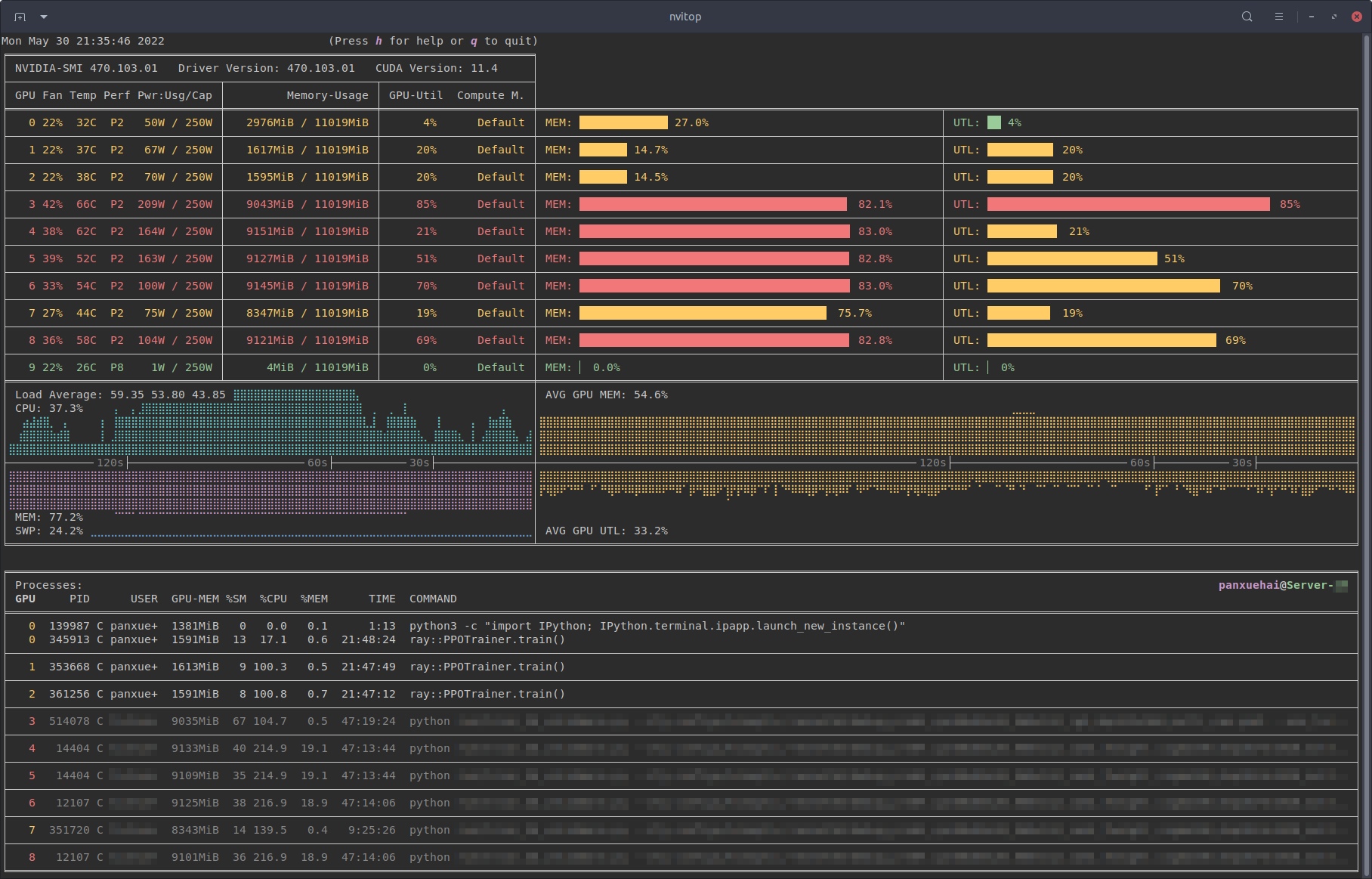
nvitop. You can always just use nvidia-smi to view the memory / power usage of your GPUs, but there are some cool alternatives that are prettier and more customizable. I pretty much use nvitop as an nvidia-smi replacement, but there are a lot of other features they have in their GitHub that you can play with.

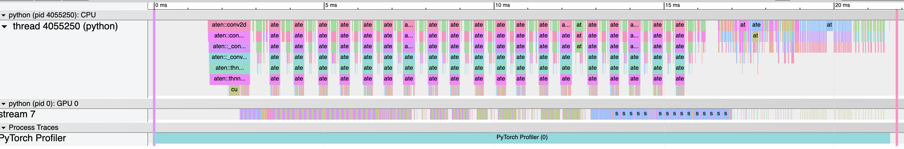
Pytorch Profiler. PyTorch has a simple profiler that you can wrap around your code for viewing the individual kernels / CPU calls. It also has peak memory usage / compute time statistics that it prints out for you, and is relatively simple to insert into your code for debugging.

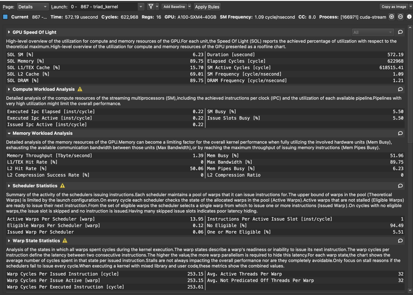
Nsight Compute and the Nsight Compute CLI (ncu) are excellent profiling tools for your CUDA kernels. It provides analysis on potential bottlenecks, as well thread, memory, and kernel call information at a very fine granularity. It also provides thorough analysis and recommendations for fixing bottlenecks in your kernels.

Nsight Systems is designed for profiling entire workloads (CPU, GPU), and is more similar to the PyTorch profiler tool.

A.5: “From scratch”-style tutorials.

It was always nice to get your hands dirty when learning a new topic. The machine learning community has made a lot of nice libraries for practitioners to use that lets you load and use a powerful LLM with a few lines of code. However, because the field moves so fast, it is a valuable skill to know what’s going on under the hood. Here, we list many useful resources for learning from the ground up (many of which come from Andrej Karpathy).

• Karpathy’s Neural Networks: Zero to Hero Playlist. Probably one of the most information-dense tutorials for how LLMs are coded from the ground up. I find his teaching style quite fun, and I think these are worth following in your free time.
• Programming Massively Parallel Processors Lectures. The PMPP book is one of the most iconic for understanding common GPU programming primitives. The lectures are from one of the authors, and they’re extremely well-made. Most of the examples are in CUDA, which is perfect for getting into efficient deep learning.
• PyTorch internals. I’m not sure how much PyTorch has changed since this blog came out (there’s slides out there for PyTorch 2.0), but this blog has a lot of nice visuals that explains how PyTorch implements tensors, autodifferentiation, and kernel dispatches.
• Optimizing CUDA Matmul from Scratch. I love this blog — the goal is to get to CuBLAS-level performance with raw CUDA, and they use a lot of the tricks and primitives you learn from the PMPP book. I found this blog to be one of the most helpful hands-on tutorials for getting started with CUDA.
• Colfax CUTLASS. Colfax has a bunch of nice blogs on GPUs, but their CUTLASS GEMM series is extremely new and well-made. This resource is probably the most up-to-date out of the ones listed so far.
• Han Song’s Efficient ML Lectures. Professor Han Song is one of the leading figures in efficient ML, and his course is freely available on YouTube. I watched the 2023 iteration of the course, but a lot of the topics center around his research which is pretty cool!
• PyTorch Performance Guide. High-level overview of common training techniques for PyTorch workloads.

A.6: Designing deep learning clusters and network topology.

We can design all the algorithms we want for working with multiple nodes, but if our cluster is poorly designed, we are strictly bottlenecked by speed. Ideally, we would want every device and node to share the same pair-wise communication latency, but in practice this is almost impossible.

NVIDIA DGX servers. NVIDIA has packaged up their GPUs nicely into these super expensive multi-GPU servers that you can plug into your cluster. They handle stuff like optimizing the inter-GPU interconnects and attaching a host processor for youA lot more details about each generation of these servers can be found here: https://training.continuumlabs.ai/infrastructure/servers-and-chips/nvidia-dgx-2. While researching this topic (e.g. when someone says they’re using a 8xH100, what else is there other than the H100s), I came across a bunch of other bundled up servers like Arc Compute and Lambda Hyperplane from third-party distributors.

Network topology. I heard this work thrown around a lot, and it sort of confused me what the relation was to say point-set topology. But network topology is literally the physical connections between nodes and devices within a cluster. Unfortunately, I know little about the design decisions here other than something of the form “node A has a limited number of lanes/ports, so we can’t just jam all the nodes together”. I hope to expand this section and add it to Part III!

A.7: Useful surveys on efficiency.

Part of the difficulty of research in this field is sifting through the sheer number of different papers. This post hopefully serves as a strong filter for many of these works, but perhaps for some readers it is too strong of a filter. Below, I list some comprehensive surveys to find more interesting works related to efficiency.

Acknowledgements

I am open to suggestions and edits, even those that are critical. I want to log these edits and changes made over time in this section to give credit where credit is due!

Citation

Just as a formality, if you want to cite this for whatever reason, use the BibTeX below.

@article{zhang2024efficientdl,
  title   = "A Meticulous Guide to Advances in Deep Learning Efficiency over the Years",
  author  = "Zhang, Alex",
  year    = "2024",
  month   = "October",
  url     = "https://alexzhang13.github.io/blog/2024/efficient-dl/"
}